T3RRA Operator's Manual

No part of this publication may be reproduced, transmitted, transcribed, stored in a retrieval system, or translated into any language or computer language, in any form or by any means, electronic, mechanical, magnetic, optical, chemical, manual, or otherwise, without the prior written permission of T3RRA Pty Ltd.

Trademark Notice

T3RRA Cutta™, T3RRA Plane™, T3RRA Ditch™, T3RRA Survey™, T3RRA Apply™, COMMAND™ and Level COMMAND™ software images and their logos are the exclusive trademarks of T3RRA. All other trademarks, service marks, software images and logos used in this documentation belong to their respective owners.

Notice of Liability

The information in this document is distributed on an ‘as is’ basis, without warranty. While every precaution has been taken in the preparation of this manual, neither the authors nor T3RRA shall have any liability to any person or entity with respect to any loss or damage caused or alleged to be caused directly or indirectly by the instructions contained in this book or by the machine-control systems and associated equipment products described in it.

Disclaimer

We make a sincere effort to ensure the accuracy of the material described herein; however, T3RRA makes no warranty, expressed or implied, with respect to the quality, correctness, reliability, accuracy, or freedom from error of this document or the products it describes. Data used in examples and sample data files are intended to be fictional. Any resemblance to real persons or companies is entirely coincidental. While reasonable effort has been made to ensure the accuracy of this publication, T3RRA assumes no responsibility for errors or omissions, or for damages resulting from use of the information contained within this manual. Information contained within this manual was current at the time of publication.

1. General

About Our Software

Both Mark Twain and Will Rogers shared a wise sentiment: “Buy land, they’re not making it anymore”. We can’t help you buy land, and we definitely can’t help you make more of it. What we can do is help you make your current land better.

This manual describes the operation of the software solutions we offer specifically for in-cab design and implementation of landforms to improve field terrain. There are many reasons to change the surface contours of a field. Most relate to facilitating efficient irrigation, or improving drainage. Further benefits relating to trafficability and enhanced management opportunities nearly always accrue.

In order to address diverse market requirements we offer several different software packages. Our most fully featured product is T3RRA Cutta. This application includes all the functionality we offer for full field landforming, ditch creation, and levee delineation. T3RRA Ditch offers all the ditch and levee creation capabilities of T3RRA Cutta but is not appropriate for users who intend to do full field earthworks. T3RRA Plane is for Best-fit full field design projects. T3RRA Apply is used to survey and apply dirt moving projects without the design step. T3RRA Survey is used solely for gathering elevation data.

Note that we also offer a related desktop design product - T3RRA Design. This product is a more traditional “keyboard and mouse” application for use in an office environment. The advanced nature of T3RRA Design requires a wholly separate manual and users should refer to it for more information.

It’s important to understand that T3RRA Cutta, T3RRA Ditch, T3RRA Plane, T3RRA Apply, and T3RRA Survey are all built using the same basic building blocks. They share many of the same user interface screens and functionalities. In this manual we will use the generic term “T3RRA software” when the topic or concept we are referring to is common to all five applications. When the information is specific to one or two of the applications this will be noted and the software will be referred to by its actual name.

1. General

Intended Use

T3RRA In-cab Software is intended for use on supported construction, landforming, and earthmoving machinery equipped with compatible hardware, GNSS receivers, hydraulic interfaces, and machine sensors.

The system is designed to assist operators with terrain guidance, grading operations, surface control, and automatic implement positioning during earthmoving and landforming activities.

System performance depends on:

correct installation
machine calibration
GNSS signal quality
terrain conditions
hydraulic performance
and operator supervision

T3RRA In-cab Software is an operator-assistance and terrain-control system. The operator remains responsible for safe machine operation, terrain awareness, and final work quality at all times.

The system must only be operated by personnel familiar with machine-control systems and safe equipment operating procedures.

1. General

Choosing an In-cab Tablet PC

T3RRA in-cab software is compatible with any 64-bit Windows 11 PC, including desktop computers, laptops and tablet PCs. While the software can be operated using a keyboard and mouse, it has been designed primarily for use with a touchscreen interface.

For most installations, a Windows tablet PC provides the best balance of portability, usability and mounting flexibility within the machine cab. We recommend using the display in landscape orientation, with a screen size of 10 inches or larger for the best operating experience.

Windows tablets are available in a wide range of performance levels, durability ratings and price points. The most suitable option depends on your operating environment and business requirements. In general, tablet PCs can be grouped into two broad categories:

Consumer Tablet	Rugged Tablet
Microsoft Surface Pro	RuggON, Panasonic Toughbook
Lower purchase cost	Higher purchase cost
Designed for office/general use	Designed for industrial vehicle use
Best suited to careful owner-operators	Best suited to contractors and commercial fleets

At T3RRA, we supply ruggedised RuggON tablets because they are specifically designed for demanding in-cab environments. Their resistance to vibration, dust, moisture and temperature extremes significantly reduces hardware failures, downtime and warranty claims compared with consumer-grade devices.

Consumer tablets are fully supported provided they meet the minimum hardware requirements and remain in good working condition. Many customers have successfully operated systems such as the Microsoft Surface Pro for extended periods without issue.

However, consumer devices are generally designed for office or home use rather than continuous operation in harsh agricultural or construction environments. Exposure to vibration, dust, weather and temperature extremes can reduce reliability and service life.

When selecting a tablet, consider not only the initial purchase price but also the operational cost of unexpected downtime. Where machine availability is critical, a ruggedised tablet—or a readily available spare tablet—is strongly recommended.

Modern tablet PCs are capable of running many different applications simultaneously. To ensure reliable machine-control performance, avoid installing unnecessary software or running resource-intensive applications while operating T3RRA software. Excessive processor, memory or storage usage may reduce overall system responsiveness.

Maintain your tablet regularly. Install Windows updates, T3RRA software updates and any recommended driver or firmware updates during planned maintenance periods. Keeping the operating system and software current helps maximise system reliability and performance.

1. General

Consider the System as a Whole

Accurate machine control depends on the performance of the entire landforming system, not just the T3RRA software. T3RRA software works in conjunction with John Deere iGrade™, combining terrain design, guidance and implementation with iGrade's machine-control capabilities. Achieving the level of accuracy expected from the system requires the mechanical, hydraulic, electrical, GNSS and software components to work together reliably.

While T3RRA software is a key part of the machine-control system, its performance depends on the condition, configuration and calibration of the equipment around it. Poor machine maintenance, inaccurate GNSS positioning or incorrect iGrade™ configuration cannot be compensated for by software alone.

Before beginning work, verify that:

The machine is in good mechanical, hydraulic and electrical condition.
The implement is correctly installed and in good working order.
The RTK GNSS receiver, corrections source and (where applicable) base station are configured to provide reliable positioning accuracy.
You are familiar with the operation of the John Deere iGrade™ system.
John Deere iGrade™ has been correctly configured and calibrated.
The tablet PC is up to date, has sufficient available storage, and is free from unnecessary software that may reduce system performance.
T3RRA software is correctly installed, configured and updated to the latest recommended version.

Don't disengage your brain when engaging T3RRA software.

T3RRA software and John Deere iGrade™ are operator-assistance systems designed to improve productivity and grading accuracy. They do not replace the judgement, awareness or responsibility of the operator.

Continuously monitor machine behaviour, positioning accuracy and work quality throughout every operation, and be prepared to intervene whenever required. Failure to do so may result in reduced accuracy, unsatisfactory work quality or unsafe operating conditions.

1. General

How T3RRA Software Works with John Deere iGrade™

John Deere iGrade™ is an integral part of the T3RRA machine-control solution. While T3RRA software provides terrain design, guidance and implementation functionality, John Deere iGrade™ performs the hydraulic machine control required to operate the implement.

Because both systems work together, the performance of T3RRA software is directly dependent on iGrade™ being correctly installed, configured and calibrated. If iGrade™ is not operating correctly, T3RRA software will not be able to achieve reliable machine control.

John Deere provides comprehensive documentation covering the installation, configuration and operation of iGrade™. Rather than duplicate that information, this chapter explains how T3RRA software interfaces with iGrade™ and highlights the settings required for reliable operation. For detailed information regarding iGrade™ operation, configuration or troubleshooting, always refer to the official John Deere iGrade™ documentation or contact your local John Deere dealer.

Verify iGrade™ First

Although T3RRA software relies on iGrade™, the reverse is not true—iGrade™ can operate independently of T3RRA software.

When commissioning or troubleshooting a system, first confirm that iGrade™ is operating correctly on its own. Once normal iGrade™ operation has been verified, configure and test T3RRA software. This approach greatly simplifies fault finding and helps isolate whether an issue originates within iGrade™ or the T3RRA software.

Communication Between T3RRA and iGrade™

T3RRA software communicates with John Deere iGrade™ through the iGrade™ Remote Control Harness. For communication to operate correctly, the serial communication settings of both systems must match.

If an iGrade™ UCC1 controller is used, configure:

Baud rate: 38400
NMEA output: GGA & GSA
Update rate: 5 Hz

If an iGrade™ UCC2 controller is used, configure:

Baud rate: 115200
NMEA output: ALL
Update rate: 5 Hz

Important: Ensure that the hydraulic threshold setup, and TCM calibrations on iGrade™ have been completed correctly. If not done this will directly impact the performance of the system and the implementation of your field designs. Make sure to carefully follow the instructions in the iGrade™ user's manual. Perform the figure 8 calibration to make sure that everything is running smoothly. If in doubt, consult your dealer.

Configuring Remote Control

iGrade™ controls hydraulic implement functions through SCV1 and SCV3. To allow T3RRA software to control these functions, iGrade™ must be configured to accept remote control commands.

Configure the SCV control modes as follows:

Machine configuration	SCV1	SCV3
Single scraper (height only)	Remote Control	Not used
Dual scraper	Remote Control	Remote Control
Single scraper with cross-slope	Remote Control	Cross Slope Control

When using cross-slope control, ensure the Cross Slope Setpoint Source is configured as Remote Control.

To ensure hydraulic commands are accepted, the corresponding SCV levers in the machine cab must also be placed in the Detent position.

To make sure that the SCVs will receive the commands correctly also ensure that their switches in the cab are set to ‘Detent’.

Connection Status

If iGrade™ does not receive remote control commands for approximately 5 seconds, it will automatically disengage remote control and display "No Remote Commands."

Under normal operation, T3RRA software continuously transmits remote control messages to maintain communication. If this message appears during operation, investigate the communication link between the tablet PC and the iGrade™ controller.

GNSS Connectivity

Although only T3RRA Cutta and T3RRA Ditch transmit remote control commands to iGrade™, all T3RRA software applications can receive GNSS position data.

T3RRA software may obtain GNSS data either from John Deere iGrade™ or directly from another compatible GNSS receiver, depending on the system configuration.

Important
Before beginning an implementation operation, use Zero Error in iGrade™ to set the current blade height as zero. Whenever zero is reset within T3RRA software, the corresponding iGrade™ offsets should also be reset to ensure both systems remain synchronised.

1. General

System Startup

Starting T3RRA Software

On most installations, T3RRA software is configured to start automatically when the tablet PC boots. If the software does not start automatically and you would like this functionality enabled, refer to the accompanying troubleshooting guide for configuration instructions.

If T3RRA software has not started automatically after Windows has finished loading, launch it manually by double-clicking the appropriate desktop shortcut.

Once started, the T3RRA software home screen will be displayed.

1. General

Installing T3RRA Software

T3RRA software is typically installed and configured by your authorised T3RRA dealer as part of system commissioning.

Before installing the software, ensure the tablet PC has a reliable internet connection and is fully updated through Windows Update. Keeping Windows current helps ensure compatibility with the latest T3RRA software releases.

System Requirements

Component	Minimum	Recommended
Operating System	Windows 10 (64-bit)	Windows 11 (64-bit)
Processor	64-bit dual-core processor	Intel® Core™ i5, AMD Ryzen™ 5, or better
Memory	8 GB RAM	16 GB RAM
Storage	256 GB available storage	512 GB SSD or greater
Graphics	Integrated graphics	Integrated or discrete graphics
Communications	USB port	Dedicated RS-232 serial port or high-quality USB-to-Serial adapter
Display	Touchscreen	High-brightness touchscreen suitable for outdoor use
Network	Internet connection for installation and updates	Reliable Wi-Fi connection for regular updates

Recommended Hardware
T3RRA recommends using a ruggedised Windows tablet PC designed for in-cab operation. Rugged tablets provide improved resistance to vibration, dust, moisture and temperature extremes, resulting in greater reliability and reduced downtime in demanding field environments.

Preparing a Tablet for In-Cab Operation

For the best in-cab experience, we recommend the following Windows settings:

Set Power & Sleep to Never to prevent the tablet from entering sleep mode during operation.
Disable Connect automatically for saved Wi-Fi networks that are not regularly used in the field.
Set the display brightness to an appropriate level for outdoor visibility.
Enable Automatically hide the taskbar in both desktop and tablet modes to maximise available screen space.

Many of these settings can be configured automatically during installation using the Tablet Optimisation page of the T3RRA installer.

Software Updates

After installation, ensure the latest version of T3RRA software is installed before beginning work.

To check for updates:

Open Settings.
Select the Application tab.
Click Download Updates.

Antivirus Software

Some antivirus software may prevent T3RRA software from installing or operating correctly.

If antivirus software is installed, add the T3RRA installation folder to the antivirus exclusion list. Refer to the troubleshooting section if installation issues are encountered.

Starting T3RRA with Windows

T3RRA software can be configured to start automatically whenever Windows starts.

To enable or disable this feature:

Open Settings.
Select the Application tab.
Open the Setup section.
Enable or disable Start T3RRA when computer starts.

1. General

Updating T3RRA Software

T3RRA regularly releases software updates to improve reliability, introduce new features and enhance compatibility with supported hardware. Keeping your software up to date ensures you have access to the latest improvements and bug fixes.

Checking for Updates

Each time T3RRA software starts, it checks whether a newer version is available. This check only occurs when the tablet has an active internet connection.

If an update check is performed, a brief notification will appear in the lower-left corner of the main window indicating either:

Your software is already up to date.
A newer software version is available for download.

Installing an Update

To manually check for and install updates:

Open Settings.
Select the Application tab.
Click Download Updates.

If an update is available, it will begin downloading immediately.

A progress window will display the download status. Once the download is complete, you will be prompted to close and restart T3RRA software to complete the installation.

Important: Before restarting the software, ensure any work in progress has been saved. A reliable internet connection is recommended when downloading updates.

When Should You Update?

As a general rule, avoid updating software while actively working in the field.

Before the start of an earthmoving season.
Between jobs.
When advised by your T3RRA dealer or support representative.
When an update addresses a problem you have experienced or introduces functionality you require.

If your current software version is operating reliably and no update is required for your application, there is generally no need to update immediately.

Reverting an Update

In the unlikely event that an update causes unexpected issues, previous software versions can be restored.

Software rollback should only be performed under the guidance of T3RRA or your authorised dealer. If assistance is required, please contact T3RRA Technical Support before attempting to revert to an earlier software version.

1. General

Upgrading from T3RRA Cutta V1 to V2

Transitioning from T3RRA Cutta V1 to T3RRA Cutta V2 has been designed to be as straightforward as possible. The familiar wizard-based workflow has been retained, along with the core operating principles used throughout V1. While the user interface has been refreshed, existing users should find the overall workflow familiar.

What's New?

T3RRA Cutta V2 introduces several significant enhancements while preserving the concepts that experienced users already know.

The most notable additions include:

The ability to combine different design types within separate regions of the same field.
Support for creating designs on top of existing designs.
The introduction of As-Applied functionality, allowing completed earthworks to become part of the project's working surface.

These features provide substantially greater flexibility but may require a small adjustment to established workflows.

When creating or modifying designs, pay particular attention to the surface being used as the design reference, such as the existing elevation or an existing design surface.

Understanding As-Applied

The introduction of As-Applied functionality represents one of the largest workflow changes between V1 and V2.

We strongly recommend reading the Understanding As-Applied section of this manual before using the feature. Understanding how As-Applied surfaces interact with existing designs will help avoid confusion and ensure predictable design behaviour.

If preferred, As-Applied functionality can be disabled, allowing operation in a manner similar to previous versions.

Migration Guide

Users upgrading from T3RRA Cutta V1 are encouraged to review the T3RRA Cutta V1 to V2 Migration Guide before beginning work. The guide highlights the key workflow changes and explains how familiar V1 concepts have evolved in V2.

File Compatibility

T3RRA Cutta V2 has been designed to maintain compatibility with T3RRA Cutta V1 wherever practical.

In most cases:

Projects created in V1 can be opened in V2.
Projects created in V2 can be opened in V1, provided they do not contain features that are unique to V2.

Because V2 introduces additional project layers and capabilities that are not supported by V1, some projects may not be fully compatible when opened in older software versions.

This compatibility allows V1 and V2 systems to continue working together during transition periods, provided project features remain compatible with both versions.

1. General

Glossary

As-Applied: Represents the current state of the field as work progresses. The As-Applied surface typically transitions from matching the original surface to matching the design surface as earthworks are completed. Also referred to as As-Built.

Backslope (Batter): The sloping sides of a drain or channel that transition from the surrounding ground surface to the drain invert.

Baud Rate: The speed at which data is transmitted over a serial communication link, measured in bits per second (bps). Both communicating devices must use the same baud rate to communicate successfully.

Benchmark: A surveyed location with a known position and elevation used as a reference for calibration and verification. Also referred to as a Control Point.

Bi-directional Error: A consistent but opposite vertical error that occurs when travelling in opposite directions. This can often be corrected by adjusting the system look-ahead time.

Blade Shift: The vertical or lateral adjustment of an implement blade, performed either manually by the operator or automatically by the machine-control system.

Borrow Pit: An excavation created by removing material for use elsewhere within a project.

Bulking: The process of performing the largest cuts and fills before completing final grading. Bulking prioritises productivity over final accuracy.

Burning: The process of embedding a design element into an existing surface.

Button Press: Selecting an on-screen control using the touchscreen. Also referred to as tapping.

Com Port (Serial Port): A hardware communication interface used to exchange serial data between devices. COM ports may be physical connectors or virtual ports created by USB-to-Serial adapters or internal hardware.

Control Surface: The reference surface used by the machine-control system to determine the required implement position. This may be an existing terrain surface, a design surface or an As-Applied surface, depending on the operation being performed.

Cross Slope: The slope perpendicular to the primary direction of travel. Cross slope is used to define the side-to-side inclination of a surface.

CSV (Comma Separated Values): A text-based file format used to store tabular data. CSV files can be opened using spreadsheet applications or text editors.

Cut Area: A region where material must be removed to achieve the target surface.

Cut/Fill Map: A colour-coded map showing the difference between the original surface and the design surface.

Cut/Fill Ratio: The ratio between the volume of material excavated and the volume required after placement and compaction. For example, a cut/fill ratio of 1.2 indicates that 1.2 m³ of excavated material is required to produce 1.0 m³ of compacted fill.

DEM (Digital Elevation Model): See Digital Elevation Model.

Design Surface: A digital model representing the intended finished terrain after earthworks have been completed.

Detent: A John Deere hydraulic control mode that enables iGrade™ to accept remote control commands from an external system such as T3RRA software.

Digital Elevation Model (DEM): A digital representation of terrain elevations across an area. DEMs are used for surveying, design and machine-control applications.

Dynamic Blade Limit: A T3RRA feature that limits cutting below the As-Applied surface to help prevent over-cutting and maintain the intended design.

Feather: To gradually blend one surface or design into another, creating a smooth transition.

Fill Area: A region where material must be added to achieve the target surface.

Finishing: Final grading passes performed to achieve the target design elevation and surface quality.

Geo-referenced: Describes data or imagery that includes geographic coordinates, allowing it to be accurately positioned on the Earth's surface.

GNSS (Global Navigation Satellite System): The collective term for satellite positioning systems including GPS, GLONASS, Galileo and BeiDou. Modern receivers typically use multiple constellations simultaneously to improve positioning accuracy.

GPS (Global Positioning System): The United States satellite navigation system. Within this manual, the term GPS is commonly used to refer to GNSS positioning unless otherwise stated.

Grade: The required elevation or slope at a particular location relative to the design surface.

Haul: The process of transporting excavated material from one location to another.

Heading: The direction in which the machine is travelling or pointing, typically expressed in degrees relative to north.

Implementation: The process of constructing the designed terrain by moving material to match the target surface.

Importing/Exporting Dirt: Importing refers to bringing material into a project area from elsewhere. Exporting refers to removing material from the project area for use or disposal elsewhere.

Land Forming: The process of reshaping terrain using curved or variable surfaces to improve drainage, irrigation or productivity.

Land Levelling: The process of reshaping terrain using predominantly planar surfaces to improve irrigation or drainage.

Look-Ahead: A control parameter that predicts machine movement and commands hydraulic adjustments slightly in advance to improve grading performance and reduce control error.

Machine Control: The combination of hardware and software used to automatically or semi-automatically position an implement according to a target design.

NMEA (National Marine Electronics Association): A communications standard commonly used to exchange GNSS and navigation data between devices.

On-Grade: The condition where the implement cutting edge is at the required elevation to achieve the target design.

Original Surface: The surveyed or imported terrain model representing the field before earthworks begin.

Pixel: The smallest element of a raster surface. Pixel size determines the resolution and level of detail represented by the surface.

Primary Slope / Secondary Slope: The primary slope is the dominant direction of fall across a surface. The secondary slope (or cross slope) is perpendicular to the primary slope.

Project File: A proprietary T3RRA project file containing survey, design and project information. T3RRA project files use the .tci file extension.

Raster: A grid-based data structure consisting of regularly spaced cells (pixels), each containing an elevation value.

Remote Control: A control mode that allows an external device, such as T3RRA software, to send hydraulic control commands to a compatible machine-control system.

RTK (Real-Time Kinematic): A high-accuracy GNSS positioning technique that uses correction data from a base station or network to achieve centimetre-level positioning accuracy.

Settle (Shrink): The reduction in soil volume that occurs after material has been placed and compacted.

Slope: A measure of the rate of elevation change across a surface. Within T3RRA software, positive slope values represent downhill gradients.

Stockpile: A temporary pile of excavated material intended for later use.

Surface: A digital representation of terrain. Surfaces are typically created from survey points or raster elevation data and are used for design, guidance and machine control.

Survey Point: A recorded position containing horizontal coordinates (X, Y) and elevation (Z). Collections of survey points are used to generate terrain surfaces.

TCM (Terrain Compensation Module): A John Deere sensor integrated into StarFire™ receivers that measures machine attitude to improve positioning and cross-slope accuracy.

Time-out: A condition where communication is terminated because a device or application fails to respond within an expected period.

Topography: The physical shape and surface characteristics of an area of land.

Topsoiling: The placement of a layer of topsoil over a finished surface to restore fertile material following earthworks.

Washboarding: Repetitive vertical oscillation of an implement that produces a corrugated surface resembling a traditional washboard.

Zeroing: The process of calibrating measured elevations to the physical cutting edge of the implement. Zeroing compensates for GPS antenna offsets, implement geometry, machine setup and differences between surveying and implementation, ensuring displayed elevations accurately represent the cutting edge position.

2. Creating Projects

Main page / New Project Page

When T3RRA software is opened, the Main Page is the first screen displayed. This same screen is also shown when New Project is selected from within the Wizard.

The Main Page provides access to the primary application controls, including display settings, software configuration, the Operator’s Manual and T3RRA support tools.

Application Information

When T3RRA software is running in windowed mode, the title bar displays information about the current application and project.

Depending on the software being used, this may include:

The name of the currently loaded project file.
The T3RRA application name, such as T3RRA Cutta, T3RRA Ditch, T3RRA Plane or T3RRA Survey.
The installed software version.

Full Screen Mode

Select Full Scrn to switch between full-screen and windowed operation.

Full-screen mode maximises the available display area for T3RRA software. Windowed mode may be useful when you need to access another application or Windows function at the same time.

If a keyboard is connected, press F11 to switch between full-screen and windowed modes.

Display Modes

T3RRA software provides three display modes to improve visibility under different operating conditions:

Mode	Description
Day	Standard light interface with a white background. This is the display mode used throughout this manual.
High Contrast	Uses an inverted colour scheme to improve visibility in some lighting conditions.
Night	Uses a dark background with a green foreground to reduce screen brightness during low-light operation.

Settings

Select Settings to review and configure the application.

Before beginning work, confirm that the software has been configured correctly for the machine, implement, project and GNSS system being used.

The available settings and their functions are described in the Settings chapter of this manual.

Open Manual

Select Open Manual to access the T3RRA Operator’s Manual.

The first time this option is used, T3RRA software will download and install a local copy of the manual on the tablet. Once installed, selecting Open Manual will open the manual directly.

An internet connection is required when downloading the manual for the first time.

Report

Select Report to open the T3RRA bug report and feature request window.

This tool can be used to:

Report unexpected software behaviour.
Submit information about a problem.
Request or suggest new functionality.

The Name and Email Address fields are automatically populated using the details associated with the software licence.

An active internet connection is required to submit a report.

2. Creating Projects

Importing External Files

T3RRA software uses the T3RRA Project File (.tci) as its native project format. Data from supported external file formats can be imported and converted for use within a T3RRA project.

To import external data, select Import from the Main Page and choose the appropriate file or data source.

T3RRA Design provides additional import and conversion capabilities and can be used to prepare many other file formats for use with T3RRA software.

Supported Import Formats

The available import options depend on the type and source of the data.

Survey and Elevation Data

Data Type	Supported Formats / Sources
Drain Paths	CSV (`.csv`)
	PCTXYZ
Full Field Surveys	CSV (`.csv`)
	PCTXYZ
	John Deere RCD Log
	John Deere ADAPT Log
	John Deere SWM Survey
	MyJohnDeere Field Operation*
Survey Data	KML (`.kml`)

*An internet connection is required when importing from MyJohnDeere.

Digital Elevation Models

JSONGrid
ESRI ASCII
Field Level II
AGPS Design File
Trimble Grid (.xyzout)

Control Files

Data Type	Supported Format
Drain Paths	John Deere Ditch Tracks (SWP Ditch Tracks)
Full Field	Field Level II

2. Creating Projects

Importing Data

T3RRA software uses the T3RRA Project File (.tci) as its native project format. Data from supported external sources must be imported using the Import function before it can be used within a T3RRA project.

T3RRA Design provides additional import and conversion capabilities and can be used to prepare many other file formats for use with T3RRA software.

T3RRA Apply does not support data import. T3RRA Apply can only work with designs created in, or provided by, other T3RRA projects.

Loading vs Importing

Throughout T3RRA software and this manual, loading and importing refer to two different operations:

Loading means opening an existing T3RRA .tci project file.
Importing means bringing data from an external or third-party source into a T3RRA project.

A .tci project can normally be loaded directly. Importing external data may require additional steps because T3RRA may need information about the source data, or the data may need to be interpreted or converted before it can be used.

Importing a File

External data can be imported when creating a project or added to an existing project at any time.

1. Open the Import Window

Select Import from the Main Page or from the Collect step of the Wizard.

If a keyboard is connected, press Ctrl+I to open the Import window.

2. Select the Import Type and File

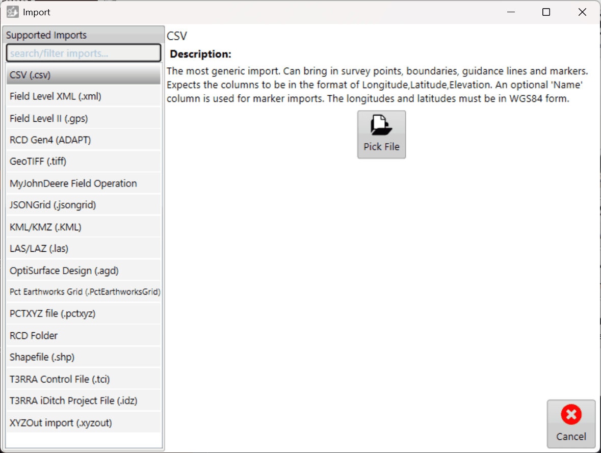
Select the appropriate data or file type from the options on the left side of the Import window.

Select Pick File, then browse to and select the file you wish to import.

3. Configure the Import

Some file types require additional information before they can be read, such as coordinate system or projection information.

Enter any required information, then select Read in the lower-right corner.

When importing CSV data containing latitude and longitude coordinates, the coordinates must use WGS84.

4. Review the Data

Once the file has been read, select the data you wish to import. A preview of the available data is displayed on the right side of the window.

T3RRA will attempt to automatically identify the type of data contained within the file. If the detected data type is incorrect, use the available drop-down menus to select the correct type.

Review the data and selections, then select Import.

5. Continue with the Imported Data

Once the import is complete, the imported data is available for use within the project. Surfacing and design operations can then be performed as required.

When elevation survey point data is imported, T3RRA automatically creates the corresponding surface.

2. Creating Projects

Loading a Project

Select Load proj. to open an existing T3RRA project (.tci). Projects can be loaded from the standard T3RRA project structure, from another location on the tablet PC, or from external storage such as a USB drive.

To begin, select Load proj. from the Main Page.

Loading from Grower/Farm/Field

Projects stored within the standard T3RRA file structure are organised using Grower, Farm and Field profiles.

Select the appropriate Grower, Farm and Field, then select the project you wish to open and press OK.

For more information about creating and managing Grower, Farm and Field profiles, refer to the relevant section later in this chapter.

Managing Saved Projects

Three management buttons are displayed alongside each project:

Button	Function
Rename	Renames the selected project file.
Delete	Deletes the selected project. Deleted files are moved to the Windows Recycle Bin.
Move	Opens the project location window, allowing the selected project to be moved to another Grower, Farm, Field or file location.

These controls allow existing project files to be organised without leaving T3RRA software.

Finding a Project Manually

T3RRA project files are standard Windows files and are not required to be stored within the default T3RRA folder structure.

To open a project stored elsewhere, select Find manually.

Use Windows File Explorer to browse to the required T3RRA project (.tci), select the file, then select Open.

This option can also be used to open projects stored on external media such as a USB drive.

Finding All T3RRA Projects

If you do not know where a project has been saved, select Show all files.

T3RRA will scan the computer's C: drive for compatible T3RRA project files and populate the project list as files are found. A progress bar in the lower-right corner indicates that the scan is still in progress.

Use the Search field to filter the results by project filename.

Once the required project has been located, select it and press OK.

Continuing a Loaded Project

Once a project has been loaded, T3RRA will open the Wizard at the appropriate stage for that project. Existing project progress is retained, allowing you to continue from where the project was previously saved.

Where the project is ready for machine control, you can proceed directly to the Apply stage.

When ready to begin implementation, select Start. You will be required to accept the displayed Disclaimer before machine control can begin.

2. Creating Projects

Saving and Auto-Saving Projects

Saving a project allows you to close T3RRA software and return to your work later while retaining the project's survey, design and other associated data.

Although T3RRA software includes an automatic backup system, regularly saving your project is strongly recommended to minimise the risk of data loss.

Saving a Project

The Save project button is available from the main Wizard pages.

Select Save project to open the project save window. T3RRA's standard project structure organises projects using the following information:

Grower
Farm Name
Field Name
Project Name

Enter the required information or select an existing Grower, Farm or Field from the available drop-down lists.

Select OK to save the project within the standard T3RRA project structure.

Saving to Another Location

T3RRA project files are standard Windows files and can also be saved outside the default T3RRA project structure.

Select Manually Choose Location to specify an alternative save location.

The save window can be navigated using either the folder tree on the left or the main file browser. Navigate to the required location, enter a filename, then select Save.

This can be used to save projects elsewhere on the tablet PC or to another available storage location.

Important — Back Up Your Projects

Regularly copy important project files to a location separate from the in-cab tablet PC. This provides an additional copy of your project data if the tablet is damaged, lost or experiences a hardware failure.

Consider backing up projects at appropriate stages throughout a job, rather than waiting until the work is complete.

Auto-Saving

T3RRA software automatically creates backup copies of project data while you are working. Autosaving helps protect against data loss if the application closes unexpectedly or the tablet PC experiences a software or hardware failure.

The autosave interval can be configured under Settings > Advanced.

Autosave files are stored in the same location as the active project and use the same project filename with an additional .backup suffix.

Recovering an Auto-Saved Project

When an existing project is loaded, T3RRA checks for a corresponding autosave file.

If an autosave exists and has a newer date and time than the saved project, T3RRA will prompt you to choose whether to load the newer autosaved version.

This allows work completed since the project's last manual save to be recovered following an unexpected shutdown or other interruption.

Manually Recovering an Auto-Save

An autosave contains the same project data format as a regular T3RRA project and can also be recovered manually if required.

Using Windows File Explorer, locate the appropriate autosave file and make a copy before modifying it. Rename the copied file by removing the .backup suffix:

ExampleProject.tci.backup → ExampleProject.tci

The recovered copy can then be opened as a normal T3RRA project while retaining both the original project and autosaved version.

3. Settings

Application Tab

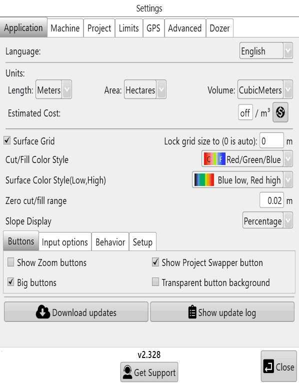
Units:

‘Language’ - Changes the language

‘Length’ - Changes unit of distance measurement.

‘Area’ - Changes unit of area measurement.

‘Volume’ - Changes unit of volume measurement.

‘Estimated Cost’ - Set an estimated cost per volume of dirt moved. To customize the currency format, click the button to the right. You can enter custom text before and after the amount. An example is shown on the right. This allows you to put your currency code and other information before and/or after the value.

Cost per cubic meter, or cubic yard (this is calculated for cuts only).

‘Surface Grid’ - Determines whether or not to show the grid lines on the map. By default the grid changes size to best fit the size of the field. Dimensions for the grid size are displayed in the lower right corner of the scanned area.

‘Lock grid size to:’ - Users can adjust grid size manually. set to 0 for auto-size.

‘Cut/Fill Color Style’ - Set colors used for Cut/Fill to Magenta/Green or Red/Green/Blue. (Magenta as cuts/Green as fills, or Red as cuts/Green as neutral/Blue as fills)

‘Surface Color Style (Low,High)’ - The surface color style allows you to change which colors represent your highs and lows. (this is limited to selecting from a drop down menu)

‘Zero Cut/Fill Range’ - Adjusting this number allows you to set a vertical range that will be considered as “on-grade”. This is a great tool for quickly identifying parts of a field with heavy earth moving. This option will not change the design height or the height of the scraper blade.

‘Slope Display’ - Show slope as a Percentage or as a Ratio. (0.1% or 1/1000)

Buttons:

‘Show zoom buttons’ - Choose to use zoom buttons for zooming in and out instead of ‘two-finger touch zoom’.

‘Big buttons’ - Check this option to increase the size of the menu buttons.

‘Show Project Swapper button’ - Choose to display the project swapper button.

‘Transparent button background’ - This setting will change the button backgrounds between gray and transparent when in design or implementation screens.

Input options:

‘Show screen keyboard’ - Choose to have the keyboard automatically open when needed.

‘Show Calculator’ - Choose to display a calculator when inputting values when needed.

Behaviour:

‘Hide buttons after delay’ - If checked buttons will fade after 15 seconds on the implementation screen. Touch screen to retrieve.

‘Collection Beep’ - Choose to enable audible notifications of collection of elevation points.

Download Updates - Choose to update to the latest version when connected to the internet.

Show update log - Lists software update details.

Set Support - helps your dealer give you remote support. You must be connected to the Internet for this to work.

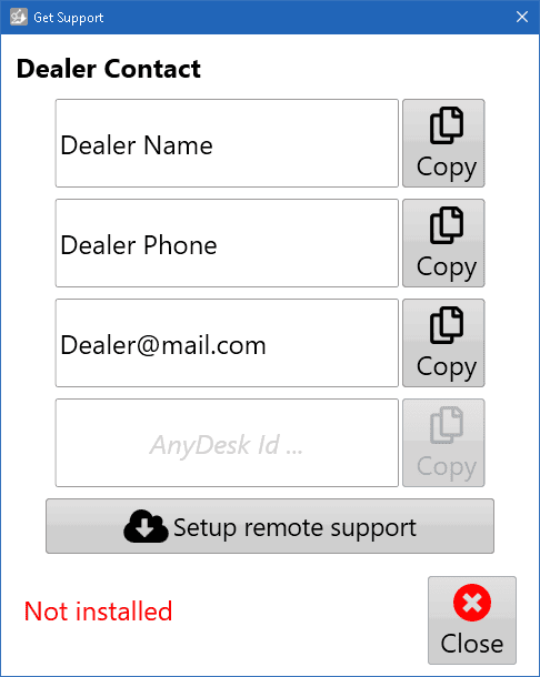
Click "Setup remote support" button.

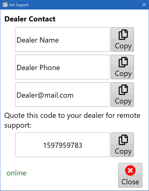
After installation, It will show a code. Your support person can use the code to connect to your computer and help get you going again. When they do, AnyDesk will open a confirmation window. Click the green [Accept] button to accept their help.

Close - Choose to save settings and exit this settings dialog.

3. Settings

Machine Tab

Look ahead delay time - In order to control blade height the software must receive an elevation from iGrade™, process that elevation, and then return a control signal to iGrade™. This control loop is quick but the time delay can cause inaccurate implementation in certain situations.

A normal “Look ahead” time is 0.3 to 0.5 seconds. The exact time is machine specific and can be determined through experimentation (see Bi-Directional error in T3RRA in the troubleshooting section). The look ahead time helps to account for the delay in the control loop.

If the look ahead time is not set the delay can cause a “bi-directional error”. This is where the blade offsets incorrectly, moving up when going down a slope and down when going up a slope. This error occurs consistently. If the look ahead time is set too LOW the implement will always grade high when going down-slope and low when going up-slope, the opposite effect will occur if the look ahead time is set too HIGH. Bi-directional error is most noticeable when working steep slopes at higher speeds.

Receiver setup - The 2 drop down menus set which sort of receiver connection is being used(left) and the number of receivers that are connected (right).

The receiver connection type in the left drop down menu has 4 options:

Auto-detect (default)
Non-IGrade
IGrade 1
IGrade 2

The number of receivers (Implements) can be adjusted using the right drop down menu:

Single
Dual implements
Two receivers on one implement
Triple implements.

T3RRA will use the front GPS receiver for any multi-bucket configuration, and both GPS receivers when set to "two receivers on the one implement".

When using multiple receivers, iGrade™ has the ability to control SCV1 and SCV3. Ensure SCV1 and SCV3 are configured correctly for remote control commands by placing them in detent, for information on how to do this refer to “How we work with iGrade™”.

When utilising dual or triple scrapers on UCC2 you may need to adjust the receiver height settings in the receiver settings in the individual receiver menu in ISO Page. Refer to your iGrade Manual for instructions on adjusting individual receiver height offsets. When using multiple scrapers with UCC1, the receivers must be mounted at the same height above the blade. Also with UCC1, implement offsets cannot be entered in the display to account for mounting error.

NOTE: To lower the blade enter a higher receiver height. To raise the blade position lower the height set in the receiver setup.

'Use Tractor GPS for surveys' - Only available with iGrade UCC2. When selected, the Tractor GPS will be used for surveying when it has RTK. Otherwise, it will fall back to standard operation.

Implement width - This value reflects how wide the implement in use is and needs to be entered manually. This value is needed for ‘Cross slope’, ‘As applied’ and ‘Pass count’.

Implement settings:

Output cross slope commands - The amount each tap of the manual left/right cross slope adjustment buttons causes the cross slope to change by during implementation. Uses percentages (not degrees).

Cross slope nudge increment - This specifies the incremental amount each press of the left and right tilt buttons will add to the cross slope.

Blade positioning - Allows the operator to specify which part of the soil profile under the blade has priority in determining blade position. This option is only available when you have entered an ‘Implement width’ and enabled to ‘Output cross slope commands’.

Classic - This position uses the design elevation as the target elevation under the center of the blade, and the cross-slope is determined by the design elevations under the left and right points of the blade. With Classic, it is easy to over-dig when driving down the midline of ditches, or to clip the top off a bank when straddling the ridge.

Average - This position looks at the design surface under the blade and goes for the overall trend. This is great for taking any full-field design and giving you basically that. It’s not so good for abruptly changing slopes, however.

Average, on top - This position is one step up from the trend method, literally. It determines the slope in the same way as the ‘Average’ method, but it always avoids overcutting.

Snap fit - This position attempts to find the best blade position, without overcutting. If you are going over a break line, you will see the blade snap from one position to the other as you traverse the break line. What it means, though, is that you will be cutting and filling most efficiently, minimising the number of passes and risk of rework. This option has been tailored for abruptly changing slopes.

Single point - This position is what everyone seems to want − Control-by-point. In this configuration, you pick a position on the blade represented by the red arrow. That point on the blade will be at the design elevation and cross slope even if it cuts below the design elsewhere. This is envisioned to be great for digging features like V-ditches.

Enable As-applied calculations - As-applied calculations show a graphic representation of the surface's current state as work progresses. For more see Understanding how “As-applied” works

NOTE: ‘Implement width’ is required to enable the As-applied feature.

Enable Pass Count Tracking - Pass count tracking shows how many times you have gone over a particular spot, an indication of the amount of work that has been done in an area. For more see Understanding how “Pass Count” works

NOTE: ‘Implement width’ is required to enable the Pass Count Tracking feature.

Note: ‘Enable As-applied calculations’ and ‘Enable Pass Count Tracking’ are set to for each system, if a different Cutta system is used your setting won’t be remembered.

Find below answer to some frequently asked questions regarding implement profiles:

Q: Is it a requirement for everyday implementation to fill in Maximum blade clearance even if you are NOT choosing/entering an Implement Profile?

A: It is not required. It is an organizational tool to create efficiency in workflow.

Q: Does the Implement profile named "Project profile" reflect the Maximum blade clearance entered?

A: The Implement profile saved will reflect all parameters entered for that profile.

Q: Am I required to use the same RTK base station for surveying and implementing (I will be using the same implement)?

A: To benefit from the Implement profile Maximum blade clearance tool, it makes most sense to be using the same tractor, implement, and GPS base.

Q: Can I use this with drains created in Auto Drains? Pattern Drains?

A: Yes, if you surveyed with the same equipment you are implementing with.

Q: How do I disable this setting?

A: Selecting a saved profile is the best way of knowing you are utilizing the Implement Profile settings for that equipment. It does not make sense to ‘disable’ an implement profile as the settings that make up an implement profile are always going to be required.

Q: When pulling multiples, does this apply to only the implement using SCV 1? 2? 3?

A: Maximum blade clearance refers to implement utilizing SCV 1.

Q: Do I need to set zero at the first drain and then I will not need to set zero again when digging the other drains?

A: Not if you have selected a saved profile and both surveyed and implemented with the same equipment. You will need to have entered or calculated the proper blade clearance.

Q: If I swap out tractors but still use the same implement, do I need to reconfigure the blade clearance distance?

A: You will need to create a new Implement Profile and name it something that describes the equipment associated with the profile.

3. Settings

Project Tab

Settings made in the project tab will not be represented in a project that is open when the settings are changed.

Surface Pixel Size - The default pixel size of 2 meters (~6 feet) should be adequate for most purposes. In some situations, it may make sense to decrease pixel size to 1 meter or even 0.5 meters (primarily to facilitate small interval contour creation, or to get good definition on drain batters/backslopes).

A field surface is represented using a “raster”. This is a grid of elevation heights. The individual cells in this grid are referred to as “pixels” and have a uniform edge size. The smaller the pixel size, the more pixels needed to cover a given area, and the more precise the elevation surface is.

Points of interest

If pixel size is too large then the field surface will not appear smooth, and short range changes in elevation may not be adequately represented.
If the pixel size is too small, then the computer will have to work harder to process the data. Dividing the pixel size by two increases the amount of pixels by four.

New Project Defaults will populate for brand new projects. Users can then choose to alter or apply them:

Project offsets

These settings allow for any GPS discrepancies to be accounted for during implementation.

The ‘North/South’ and ‘West/East’ directions to move the map (+ is North, - is South) (+ is West, - is East).

‘Implementation’ is a vertical offset used during implementation only.

3. Settings

Limits Tab

Blade Shift Increment -Used to set the height adjustment value of the up/down elevation adjustments buttons in the implementation wizard step.

NOTE - recommended distance for the blade shift increment would be 0.03 - 0.06 feet (0.4 - 0.8 inches, or 0.01m - 0.02m).

Static Blade Limit - This feature allows you to temporarily alter your target design heights by a certain amount. For instance, by setting the Static Blade Limit to 50% you will effectively be setting your target cut and fill heights to be 50% of what the actual design calls for. This setting can also be used to overfill a design by a percentage to allow for soil to “sink “ by a percentage over time. Having a setting of 110% will fill a 100mm fill to 110mm to allow for future compaction.

This is useful for building up banks, roads, or mounds in gradual steps and allows for even compaction of dirt.

The checkbox 'Ignore cuts' is useful if you want to gradually build up a mound of dirt by using the vertical nudge to lower a design surface below the current surface and then slowly nudge it upwards so that the fill pattern starts with the apex of the mound and proceeds outwards. In this case you do not want to cut in the regions where the mound design surface is currently nudged below the original surface. NOTE: 'Ignore cuts' can be activated even if the Static Blade Limit is set to “None”.

The static blade limit amount is set on the implementation screen.

Methods to progressively add layers of dirt to a fill area.

Static Blade Limit

by Percent

Static Blade Limit

By Absolute Value

Combination of vertical blade offset

+ Ignore cuts

Dynamic Blade Limit - The increment which the blade will move per pass of cut or fill. It allows progressively cutting to a total depth without over cutting on an individual pass.

This feature is designed to allow cuts to be taken in “bite size“ chunks without causing the machine to be overloaded.

It can optionally be applied only to cuts, only to fills, or both.

It uses the as-applied functionality to track blade heights on previous passes in order to set the current blade height. Dynamic Blade Limit does not operate unless as-applied functionality is activated. For more see Understanding the relationship between the “As-applied” surface and the Dynamic Blade Limit.

3. Settings

GPS Port Settings Tab

GPS - Displays the COM port that is used to communicate with the GPS. Ensure you have selected the correct port with the drop down menu.

Baud (Rate) - The communication speed between the software and GPS (it should match the baud rate of the GPS).

Scan for GPS - Checks the available COM ports and usual baud rates for valid GPS data.

Warning/Error Configuration - Settings changed on this page will stay even after the system is turned off.

Current - Displays the most recent GPS information received in a table.

Raw GPS data - Displays the most recent GPS data received. Primarily used for diagnostics, should support be required.

Output Data - Displays the most recent outgoing communications. Primarily used for diagnostics, should support be required.

Recent GPS errors - A list of the most recent GPS errors, for review in case they are intermittent.

Open Device Manager - Used to investigate COM port issues if required.

Connect and Disconnect - Manually start or stop communication with the app controller.

NOTE: T3RRA software and iGrade™ must have identical Com port and Baud Rate settings in order to communicate.

3. Settings

Advanced Settings Tab

'Enable GPS data log’

It is highly recommended to keep this enabled. The GPS data log is sent along with error reports to assist in finding a solution.

‘Enable diagnostic data’

It is highly recommended to keep this enabled because the data collected is valuable for us in assisting you if any issues should occur.

‘Open Task Manager’ will open the computer's task manager tool. This will display all current systems running on the computer.

‘Explore error logs area’ will open the windows folder on the tablet that contains all error log files. If you encounter an issue we recommend you send us the latest file so we can find the cause and correct it quickly.

‘Version Manager’

Allows the software version to be downgraded if you are experiencing a particularly bad error. It is highly recommended that a support request be added if you use this.

‘Disable serial mouse’

If your cursor is jumping around the screen or you are getting “COM in use” errors it can be corrected by disabling the serial mouse.

‘Reset to Default’ This will reset all settings to Default.

‘1Hz, 5Hz, 10Hz’ Send Messages to iGrade to control the output rate of GPS NMEA data. This function is experimental and should only be used if you accept that the system may not behave as expected, these button may also be removed in future versions.

‘Automatic backup frequency’ This drop down menu allows you to change the frequency at which the T3RRA Software backs up your work. The available options are Never, Low, Medium, High.

‘Terrain model Quality’ This setting is set to High by default and most visible when looking at surfaces in 3D. Lowering the setting some details may appear to smooth out, details and depressions are still there but are not represented in the 3d display.

‘Map update rate’ This will alter the rate of the map updates during Surveying and Implementation.

4. Wizard

The T3RRA Wizard

The ‘Wizard’ is home to the primary functions of T3RRA software and the place where you will find the tools used to survey, design, and implement.

The wizard will guide you through the 4 logical steps involved in the T3RRA software process.

If you need to start a new project you are able to return to the ‘Main Page/New Project Page’ by pressing the ‘New proj.’ button found in the top left corner of all wizard pages.

T3RRA Survey does not have ‘Design’ or ‘Apply’ (Implementation) wizard steps. Sections in this manual relating to these are not relevant to T3RRA Survey.

4. Wizard

Common tools found in the Wizard

There are several buttons that can be found on many wizard pages.

Zoom Controls
Choose Model/Layer
Image Overlay
GPS Controls (limited to surveying and implementation)
Markers (limited to surveying and implementation)
Start, Stop, and Pause commands (limited to surveying and implementation)
Delete Drain (limited to surveying and surfacing)
Extend Drain (limited to surveying and surfacing)
Split Drain (limited to surveying and surfacing)
Delete Points (limited to surveying and surfacing)
Tracking Options (limited to surveying and implementation)
Screenshots
Battery power indicator

4. Wizard

Zoom Controls

There are multiple methods available for zooming your map.

The first method that can be used is the 2-finger pinch controls. By pinching your fingers together on the screen you can zoom out and by moving your fingers apart you can zoom in.

The alternate method is the use of zoom in and zoom out buttons that can be added to the bar along the top right.

The zoom buttons are not shown by default. To enable these buttons check the 'Show zoom buttons' box under ‘Settings > Application’.

Independent of these zoom controls is the 'Zoom to full' button, this button does NOT need to be enabled. When pressed the button zooms the map in or out to the maximum size that shows the entire surface grid of the map.

4. Wizard

Image Overlays

‘Image overlays’ allows geo-referenced image data to be imported into a field.

The image overlay is accessed by pressing the button at the top of the screen (Shown right).

Add image

This is the primary method for adding overlay images to the field. When the button is pressed a file window will open to select the desired file. The file types that are currently supported as overlay images are .KML and .TIFF.

Load image from JDOC

Images from the John Deere Operations Center can be downloaded into the image overlay. This is useful for comparing previous data (such as yields) with current survey data.

Delete images

Overlay images can be deleted by unchecking the box next to them and pressing the ‘delete images’ button. This will delete the layer from the available list.

Transparency

Overlay images can be set to be transparent so that layers below them can be seen. Check the box to the left of the layer and then press the transparency button on the right side.

Layers

Pressing on any of the layers will cause it to be displayed over the others.

4. Wizard

Choose Mode/Terrain/Layer

Mode

2D View - By default the map will be displayed in a 2D aerial view.

3D View - When switching to 3D view the map will show all the terrain as small hills and valleys. In this viewing mode if you press the vertical scale magnifier (shown here) it will increase the exaggeration of these hills and valleys so that they can be more easily identified. The focal point when viewing in 3D can be changed by quickly double tapping on a position.

View

When viewing a map you have a variety of display options.

Surface

This refers to the source for the 3D topography and coloring of the map. There are 6 options:

Elevation - This terrain viewing mode shows the map as the original surface prior to any dirt being moved. Displays the map in a Red to Blue gradient scale with Red being low areas and Blue being high areas.

Design - This viewing mode shows the design that has been applied. This is the surface that you are attempting to reach at the end of the dirt moving process. Has the same color scheme as Elevation.

Cut/Fill - Shows where the design will be taking dirt from and where it will be putting it. Coloring of this layer depends on the current Cut/Fill color scheme (Settings > Application).

As applied - Displaying the map using this method shows changes as they occur. It shows a real-time representation of progress as work progresses. Has the same color scheme as Elevation. This terrain is only available if ‘As Applied’ mapping has been enabled in the machine tab of ‘Settings’.

As Cut/Fill - Shows where the design will be taking dirt from and where it will be putting it. Coloring of this layer depends on the current Cut/Fill color scheme (Settings > Application).

Pass Count - This layer displays how many passes you have done over an area. This layer is only available once pass count tracking has been enabled in Settings > Machine:

Layers

Various defined layers can be turned on and off here. This includes the current surface (see above), depressions, drains, linework, and overlays such as KML that have been loaded. The buttons at the top allow you to load and clear layers, and beside each layer is a transparency toggle button. Click the button to change its transparency.

NOTE: The depressions layer is not shown if the project only has drains (and no elevation surface).

4. Wizard

GPS Data

In the lower right corner of the screen is the GPS information button. It displays the latitude and longitude of your current position as well as your current heading.

TIP: Right clicking (press and hold) on this button will reveal a context menu with the option to display coordinates in UTM format.

When you press this button the ‘GPS Info’ window will open with more detailed GPS information.

This window provides the following information:

Serial port parameters: displays the current settings for the com port and baud rate that is being used. There are flashing arrows which indicate that the software is sending and receiving information.
Warning Thresholds: used to set limits for certain parameters. When these thresholds are being approached the borders of the screen will flash orange, once any of the thresholds have been exceeded or connection to GPS is cut the borders of the screen will flash red.
Output: shows all the GPS information currently being received.

Serial port parameters

Com port: The Com port # is assigned by the adapter. In the drop down box you can find all available com ports. It is important that this is set to the serial port that is physically attached via cable to the iGrade™ Application Controller. Diagnostic information about current serial ports can be found in the Windows Device Manager. One way of accessing this Windows tool is via the button in bottom left of ‘Settings > GPS’ .

Baud rate: The speed at which the system talks to iGrade™. It is important that this matches the iGrade™ settings or the T3RRA software will not be able to talk to iGrade™. We recommend setting the baud rate to 38400 when connected to iGrade v1. If connected to iGrade™ v2 we recommend setting the baud rate to 115200 with NMEA Message Type set to “All”.

Warning Thresholds

Idle timeout: If no GPS messages have been received in this time period an error warning will show.

RTK Timeout: This monitors the time since the last good RTK correction packet was received. It should not normally be set above 10-20sec.

Max VDOP: Vertical Dilution of Precision is a measure of the altitude accuracy. For the most accurate implementation you will want this value as low as possible however setting lower than 2 may cause interruptions in the use of T3RRA software.

Min Satellite Count: Sets how few satellites the GPS needs to see before a warning is shown.

Output

Current & Raw GPS Data: Current displays the current position data for the receiver, while Raw GPS Data will display all the messages that are coming in.

Lat & Lon: Your current location coordinates (latitude and longitude).

Altitude: Your current height (Displayed in chosen measurement format) above sea level.

Num Sats: The number of satellites that your GPS is currently tracking. This is linked to the Min Satellite Count in Warning thresholds and provides an error if this number drops below what is set there.

Fix: The type of position solution calculated.

Time: The current GPS time.

Last Correction: Time since receiving the last differential correction message from the base station. Should be as low as possible for the most accurate readings. It is linked to the RTK Timeout in Warning thresholds and will provide an error if it exceeds that time limit.

VDOP: Vertical Dilution of Precision. If this number exceeds the value in the Max VDOP in warning thresholds it will show an error.

4. Wizard

Markers

Markers on designs allow for setting points of interest at user-selected locations. This includes using a marker as a benchmark “control point” location in the design. To use a marker as a Benchmark location, refer to ‘Set Zero using a marker’ in the Implementation section of this manual.

Set marker - use this tool to set a marker on the map. Markers are always placed at the current location.

When a new marker is created a window will appear allowing a name for the marker to be entered.

Edit Marker - this opens a window that allows you to select any marker on the map and edit it.

The ‘Edit Marker’ button will open the below window allowing you to see the information of each marker that has been placed including heading, distance and height of the marker relative to your current position.

Pressing the button next to the marker name will let you change the name of the marker.

The buttons at the bottom of the window allow you to select all the markers, delete the currently selected markers, export the currently selected markers and close the window.

4. Wizard

Start, Pause and Stop controls

In the Surveying and Implementation screens the ‘Start’, ‘Pause’, and ‘Stop’ buttons are used to control the beginning and ending of the relevant activities.

These buttons do have slightly different functions depending on when they are used.

Normal function:

During normal function these buttons will act in the following way.
‘Start’ will begin the system either surveying data or implementing a design. It will also start logging path counts (if enabled). The title of the button will reflect which action it will start.

‘Pause’ is only applicable to Surveying. The use of the pause button in surveying is to allow you to continue a path after moving around obstacles. For example surveying a drain, pressing the pause button and moving then the start button will tell the system that the same drain continues where you are.

‘Stop’ will stop the surveying of the area or the implementation of a design. Using the stop button in surveying tells the system that when you press start next it is a separate area. Using the same example as pausing, if surveying a drain pressing the stop button moving and then the start button will tell the system that this is a new separate drain.

Drain Surveying function:

The ‘Start’ ‘Pause’, and ‘Stop’ buttons will change function slightly when the software is set to survey drains.

‘Start’ will start the system surveying a drain.

‘Stop’ will end the current drain survey. Pressing ‘Start’ after this will start a new drain.

Pausing collection is designed to allow for situations where the collecting vehicle cannot physically traverse a section of drain line.

4. Wizard

Drain Surveying specific edit controls

The following tools become available in the ‘Collection’ and ‘Surfacing’ stages if drain survey points exist.

Edit Drain
Merge Drains
Extend Drain
Split Drain

Edit Drain

This button allows you to edit complete drain paths from the project.

After pressing the 'Edit drain' button a window will appear with a list of available drain paths. Select a drain from the list, and press the corresponding button to either change the name of the drain or delete it.

Merge drains

This tool allows two drains to together at either end. When merging a copy of the original drains with the joining line will be made and you be given the option to delete the originals if you would like.

Extend drain

This tool allows you to arbitrarily extend a drain from either end of the surveyed path. This can be useful if the drain needs to extend to a location that was not directly accessible by the surveying vehicle.

Pressing the 'Extend Drain' button will bring up the below screen. This screen allows you to extend the drain in whatever direction you wish.

The red arrow shows the direction in which the drain will be extended, as well as which end of the drain will be extended.

Use the controls on the left hand side to select a drain. Then choose the length, elevation, and direction of the extension.

‘Rel elevation’ adds (or removes) the value entered into to the elevation of the existing drain end to calculate the elevation of the extended drain end.

‘Abs elevation’ Sets the extended drain end to the value entered.

For example, to extend the drain 1ft below an ending elevation height of 100ft:

Rel elevation value: -1ft

Abs elevation value: 99ft

Once you have finished making these adjustments press the 'Extend Drain' button.

Split drain

Split drain allows you to split a drain into two separate drains.

First select which drain it is you wish to edit from the 'Which drain to split?' drop down menu in the bottom center.

Once a drain has been selected you can press anywhere along the drain profile. A blue arrow will appear to show where the split will occur. The arrow can also be moved using the left and right arrows found to the right of the ‘Split at Distance’ option.

Create a Marker for referencing by choosing the Marker button.

Name the new drain using the 'New drain name' text box. Once you are happy with all of these settings press the 'Split Drain At Point' button to apply the split.

NOTE: The new drain name cannot be the same as an existing drain. The 'Split Drain At Point' button will become disabled in this case.

4. Wizard

2D Current Position Tracking Options

When surveying or implementing there are 4 options that control how vehicle location is tracked on the screen in 2D. The options for 2D tracking are ‘Scroll’, ‘Center’, ‘Dir. up’, and ‘Manual’.

Scroll
This option will show the GPS position indicator moving freely on the screen and will move the screen as the indicator approaches the edge to ensure that the indicator is always present on the screen.

Dir. Up

When the ‘Direction Up’ option is active the map will rotate to make sure that the direction of travel is always to the top of the screen.

Center

The Center option has 2 parts, first it locks the indicator to the center of the screen so as it moves the map moves to make sure it stays in the center. The second part is that the map is locked to always have north at the top of the screen.

Manual

This option makes it so that the system does not lock the direction of the map or fixate on the location of the indicator so that even while surveying or implementing you can inspect other sections of the map. Caution: in this mode the vehicle icon can move off the edge of the map.

4. Wizard

3D Current Position Tracking Options

When surveying or implementing in 3D there are 2 options available. The first option is ‘Follow Tractor’ and the second option is ‘Stop Following’.

Follow Tractor

This option keeps the tractor at the center of the screen at all times, the camera will be placed behind the tractor when pressed.. While in 3D viewing the camera can only be moved to view the tractor from various angles and will rotate with the tractor as the primary focus.

Stop Following

This option stops the camera from following the tractor. While using this option the tractor is able to drive off the edge of the screen and the camera will not follow it, however whenever a change is made to the camera angle it will snap back to the tractor's current position and use the tractor as the focal point.

4. Wizard

Screenshot

In the top right of any mapping window is a small button with a camera. Pressing the camera button will take a screenshot of what is currently on the screen.

After taking a screenshot a pop-up window will appear (shown below). Pressing ‘Yes’ will open the folder where the screenshot is saved.

4. Wizard

Battery Level

In the top right of the screen next to the screenshot button you will find the Battery level indicator. This indicator displays the tablet/computer's battery level and whether it is plugged into power or not.

5. Surveying

Surveying Overview

The ‘Collection’ wizard step allows you to collect elevation heights from your field. This is done to create a topographic representation of the field surface.

In T3RRA software collection is normally accomplished by driving over the surface of a field while logging GPS elevations. Once sufficient points have been collected (surveyed) they are then processed in order to create a Digital Elevation Model (see definitions). In T3RRA software we refer to this process as ‘Surfacing’ and this is performed in the next wizard step.

The key concept with surveying is: “Collect enough points to create a good surface, but no more”.

If you do not collect enough points from the field you will end up with a poor representation of the field. If you collect too many points you will have wasted time and fuel in order to create a surface that is not markedly better than one created from fewer points. As well as the number of points collected, the accuracy of the final surface depends on where the points are collected.

Getting a good representation of the field surface is not a difficult task. Getting a good surface representation while minimizing time spent doing it requires more effort and experience. Figuring out the total number of points to collect, and the best pattern to collect them in, is an art that requires experience. If you do a lot of it you will soon start to understand how to improve and optimize your surveying technique.

However, new and casual users need not despair. In general, we would advise users not to attempt to optimize this activity too much. Extra time spent getting a good survey is usually insignificant relative to the time spent moving dirt. A thorough survey and an appropriate design will save far more dirt moving time than any time added while over-surveying.

Also, be sure to read the section ‘Surveying tips’ later in this document.

5. Surveying

The 'Collect' wizard page

If you are at the Main Page and want to begin surveying first press the 'Wizard' button.

Then choose the second wizard step ‘Collect’ at the bottom of the page. This will take you to the ‘Collect’ wizard page.

You are able to import survey data from other sources as CSV for Field and Drain surveys or as KML for Boundary Surveys. Press the 'Import' button to import existing survey data in CSV format.

Hint: If you would like to examine the CSV format used by T3RRA software to import/export survey points, simply export some collected data and open the resulting file in a text editor.

To begin collecting elevation points use the ‘Start’ button (in the centre section of the screen). If data has previously been collected this will still be present when you enter the mapping screen.

We consider it best practice to drop a marker for reference prior to beginning any survey. Do this at a location you know you can return to reliably. This will assist you in shifting the survey points in the future should it become necessary to do so.

Before collecting elevation points you must decide whether you are collecting data for a full field, for a drain or a boundary. We distinguish between these three collections because the way the data is processed in subsequent steps is quite different. You can however collect drains, full field and boundary surface points at the same time by swapping between them as required. Survey modes are swapped between by pressing the survey button in the bottom right of the screen until the icon for the type of surveying you wish to do is displayed or until the text in the top left corner of the screen reads as the type of surveying you would like to do.

NOTE: Best practice is to not overlap different survey types. Instead, press Pause when traveling over different survey points then Resume once clear.

(the icons below: Field survey on left, Drain survey in center, Boundary survey on right)

To begin collection select the ‘Start’ button.

The ‘Pause’ button is used to finish data collection while moving around obstacles or avoiding replication of survey points, while the ‘Stop‘ button is used when data collection is finished.

You can edit your survey data at this point. For more information, see “Survey point edit controls”. These options are documented under the collection page, and operate the same way.

When all collection and editing of data points is complete use the 'Return' button to return to the main ‘Collect’ wizard page. You will be asked to confirm keeping changes to the elevation data.

At this point it is recommended that you save your project. If you wish to save the file externally use 'Export' step of the wizard found at the bottom of the screen. Field and Drain Surveys data will be exported as CSV files, Boundary survey data will be exported as KML files

NOTE: You should always use ‘Save proj.’ to save your T3RRA project. This saves in the native file format and is the easiest file type to reopen in T3RRA software. Exporting is optional, and depending on the type of export you perform you may not always be saving all the information that exists with your T3RRA software project.

5. Surveying

Field Surveying

When you enter surveying you will be in Field surveying mode (except in T3RRA Ditch where Drain survey mode is the default). Points that are collected in field survey mode are shown on the map as circles.

We do not require you to collect a field boundary when surveying. Some do consider it best practice to drive the perimeter of a field regardless, collecting elevation points as they go.

When surveying fields travel slowly across the field to ensure that plenty of data is recorded for an accurate representation in later stages.

Collected points can be deleted using the two available methods:

Delete in a circle.
Delete points in line.

Markers can also be placed and deleted.

5. Surveying

Magic Plane

The Magic plane is a shortcut method for creating a plane of survey points without actually having to collect them. This can be used when the grade and direction of the desired plane is known and getting accurate cut/fill volumes is not required. An example would be a building pad.

NOTE: If you use ‘Magic plane’ as your original surface you are unlikely to be able to create an accurate cut/fill map. This is because the newly created plane is unlikely to match the actual real world surface. Any cut/fill map created from a design you place on a ‘Magic plane’ will be relative to it, and not the real world surface.

Start Point - The 2 options available are center or edge, this will generate the magic plane with your current location (or the location of some pre-existing surveyed points) at the center, or at the center of an edge.

Field Length - This is the length of the magic plane and can be adjusted as needed.

Field Width - This is the width of the magic plane and can also be adjusted as needed.

Direction - This sets which direction the magic plane is oriented.

Slope Percentage - This sets the degree of the slope.

Secondary slope - This is enabled by selecting the “Enable secondary slope” check box. (the secondary slope runs at 90o to the primary)

5. Surveying

Drain Surveying

T3RRA has a drain collection mode that you must use when surveying drain lines. The button is at the bottom right of the survey collection map window.

When in 'Drain survey' mode you must drive the length of the drain in order to collect the data. It doesn’t matter whether you drive from source to outlet or vice versa. When points are collected in 'Drain survey' mode the data points are displayed as squares.

Available features:

Delete all or portion of drain line.
Extend drain’s length.
Split drains.

(see Drain specific edit controls)

After you have finished surveying:

Design drains from either direction.
Choose Best-Fit, Multi-Fit, or Linear-Fit drain design.
Add batters/backslopes to drains.
Export drains as guidance curves.

5. Surveying

Boundary Survey

Boundary surveying allows you to survey the outer perimeter of a field which can be used for Design purposes.

In T3RRA software the boundary survey mode is located in the bottom right corner of the survey screen and is accessed by pressing the survey mode button until the boundary survey mode icon is displayed and ‘Boundary’ is displayed in the top left corner of the screen.

When using Boundary survey it is not required to survey the entire perimeter of the field. If you start your system in one corner of your field but you know the position you want to start from is directly across from you, you can survey the rest of the sides of the field and the Boundary survey tools will automatically close the boundary line once you press the stop collection button.

To make a boundary with few points (as shown above), simply start collecting a boundary while stationary, then pause collection while traveling to the next corner. Once at the next corner, resume collection for a few seconds, then pause to go to the next corner. In this way you can collect a boundary with only the points you want, but you can use the delete points tools to thin out extraneous points as necessary afterwards.

There are 2 tools specific to only Boundaries: Delete boundary, and Scale the boundary.

Delete boundary: allows you to delete a specific boundary if multiple have been recorded or if you wish to start the surveying over again. Elevation points that are collected while recording the boundary will remain even after the boundary has been deleted.

Scale the Boundary: this tool allows you to expand or retract the size of the boundary lines by moving each boundary line a set distance away from the original position to a maximum of 98ft (30m) and a minimum of -98ft (-30m).

Exporting boundary information: Boundary survey information can be exported as Shapefiles or as KML files

5. Surveying

Survey Guidelines

No matter what type of surveying you are doing you are able to implement guidance lines on the survey surface by pressing the guideline button at the top of the screen.

The 'Guidance' button will cause a pop-up window to appear on the screen with a two design options for AB lines in the 'Type' dropdown menu.

The default type is 'point A + Point B' which draws AB lines based on 2 set points on the field. The location of these points can be set in 3 different ways

If you know the latitude and longitude for the points they can be input manually.
Drive to Point A and click “Set” then drive to Point B and click “Set”.
If you have recorded markers you are able to use their GPS locations for either or both of the points.

A single point can be used by selecting the 'Point A + Heading' type. Like with using 2 set points Point A can be set using the same methods mentioned above. The 2nd point is replaced with your current heading and can be adjusted to a heading of your choice.

Once the 'Type' is selected the guidelines will then create a central line from the information provided and duplicate lines parallel to it, spacing the to what has been set in the ‘Track spacing’ field at the bottom of the pop-up window.

The lines made with the guidance tool will be blue and the centre line will be red.

The nearest line to your current location will be highlighted bright purple.

As shown below when surveying a light bar at the top of the screen will display how far you are from the nearest line, which side of the line you are on, and which line you are on (e.g. E2 is 2nd line east of the centre line).

5. Surveying

Surveying Tips and FAQ

Tips for Collecting Elevation Data

Use a vehicle where the GPS-to-ground offset will remain constant (such as a tractor, truck, or ATV – not a harvester or self-propelled sprayer that will shift vertically depending on load).
If the field you are surveying has wheel ruts, either stay in them or stay out of them. Do not alternate between them.
Do not survey in fields where there will be variable wheel sinkage – ie., if part of the field is wet and part is dry.
Trace the course of any waterways and banks you want to include in the elevation model. Drive the centerlines of such features, and also drive the shoulders.
Ensure that your base station is within 1.5 miles (2.4 km) of the area you are surveying.
Areas that exhibit a rapid change in slope will need to be surveyed more intensely (closer swatch widths)
Survey at a slow enough speed so the vehicle does not rock or bounce measurably.
If you are using an implement based receiver to survey with, DO NOT alter the elevation of the implement while surveying. If using a scraper mounted receiver, raise the blade to full height before starting the survey and leave it at this position for the duration of the survey.
Save your data as often as necessary. Consider how long it would take to re-do the work you would lose if your computer crashed at any point in the survey.
Use markers to set benchmark height/control points.
Collect elevation data on 30-50ft (9-15m) passes (no more than 80ft/24m). Complete more passes in areas of the field with detailed terrain.
Try not to double survey areas. Use the pause button to skip over the already surveyed area before recommencing.
Drop markers as required.
Points are logged once every 2 meters (6.6 feet). The data received between these points will be averaged. This reduces the effect of noisy GPS (bumpy ground or bouncy implements).
Preferably use 5Hz, as it will allow us to better compensate for noisy data.

Surveying FAQ

Q: Why are there gaps in the GPS surveyed data?

A: This can be caused because the GPS has stopped transmitting (check the connection) or it can be that the user has hit “Pause” or “Stop” on the T3RRA Display. Pausing can be used when one needs to stop surveying for a time and then resume from the same point. (i.e., for a lunch break)

Q: Are there any limits on logged data?

A: We will only record a data point once every 2 meters (6.6 feet). Any data received that’s less than 2m from the last logged point will be averaged into one record.

Q: What do we mean when we say we “average” the collected data into one record?

A: If we receive a GPS read every 50cm, we get 4 GPS reads every 2 meters. We take all of those data points and average their position (latitude and longitude) and their elevation to produce the dropped point. This allows us to compensate for the fact that the surface can be quite rough when surveying.

Q: Why does the logged point always appear about 1m behind the tractor?

A: This is because of the averaging. As we average the position as well as the elevation it will drop ½ the collection distance behind the tractor.

5. Surveying

Surveying with extra sensors (T3RRA Survey only)

T3RRA Survey allows you to bring data in from additional survey types. When you hit the “start” button to begin surveying, you will be presented with various options.

Choose the first option (GPS data) if you don’t have anything additional to collect with.

After choosing your sensor, the collected elevation points will be based on the sensor, so you get a color gradient showing the collected sensor data. The “Current” in the top left of the screen will also show your current sensor value.

The GPS screen will allow you to debug the sensor data

After you’ve selected your sensor, surveying works the same as for the other tools, so read on to learn more about the available options to you.

How to export/view surveyed data

To export all the data gathered in the survey, go out to the wizard step and go to the final step “Export”. Currently, “CSV” and “PCT AgCloud” exports will allow the sensor data to be retrieved.

5. Surveying

Map: Recent GPS Errors

In the top left of the screen, after a GPS error is encountered, an INFO hint will be shown.

Tapping on this text will open the GPS info window to show the recent errors. This is helpful if you have frequent but intermittent errors that happen too quickly to read the error messages.

6. Surfacing

Surfacing

"Surfacing" is a term used to describe the process of creating a continuous map (i.e., a “surface”) from all the discrete elevation data points collected in the 'Collect' wizard step.

This is done so that every location in the field (or work area) has an elevation point associated with it, not just the places where GPS data was physically collected. The software estimates values in all the blank areas between the survey dots.

For every blank position on the map it looks a set distance in every direction to find actual surveyed points. This distance is called the ‘Search radius’. Once it finds enough points it will estimate the blank location based on these points.

Upon exiting the 'Collect' step, T3RRA will attempt to automatically calculate the best search radius and create a surface from the collected data. If you wish to view the surfaced data before going to the ‘Design’ wizard step, pressing the 'Surface' wizard button (at screen bottom) will allow you to both view it and make manual changes (if it does not match your expectations).

NOTE: If you make a change to the collected elevation points (for example: by deleting a drain) you should re-run the surfacing step.

6. Surfacing

Setting the Search Radius Manually

If the automatically generated search radius does not achieve what you expect it is possible to manually adjust the search radius in the bottom left corner of the surfacing page. There are a few things to take into account when manually adjusting the search radius.

When converting discrete elevation points into a continuous surface, a ‘Search radius’ is required. To estimate the elevation at any point on the surface which was not directly measured, we look at the surrounding measured points. The distance the surfacing algorithm will look for surrounding points is determined by the search radius.

Gaps will appear on the surface if the search radius is smaller than required. There is normally no visible effect on the resultant surface if the search radius is larger than required (although the surfacing will take longer to complete). In some instances surface artifacts will occur where the surface bridges across sections of the field where you would not expect it to. Examples might be a pond in a field, or the inside corner of an “L” shaped field. You can sometimes remove these areas by choosing a smaller search radius. Normally the effect of these artifacts is not great, although they can have impacts on your area and dirt volume records.

In general, a search radius should be about 2 times the swath width at which the data was collected. This sizing should ensure that the time it takes to apply the surface is still short but that as much data as possible is used to generate a representative map.

6. Surfacing

Inline Offset

'Inline Offset', also known as 'Fix Lag', is a surfacing tool that assists in making corrections to elevation data that is imported from other sources.

To access this tool press the ‘Fix Lag’ button located at the left end of the tools at the bottom of the screen. Pressing this button will open a pop-up window that will provide you with the options to correct elevation alignment.

When correcting elevation data adjustments will be updated in real time on the map.

This will help to make sure that the changes you are making are correct before accepting them. There are 2 settings that control the correction of elevation data.

'Shift distance' moves the data points along the recorded path and can only adjust data to a maximum distance of 30m/100ft. The distance can be manually set or adjusted using the slider.

'Pass Separation' is how far must be between any point and the next point along before it is considered to be a new segment. There is no limit to this distance.

When making changes to the data in the inline offset window they will be reflected on the surface on the map - Check that your change has the desired effect before accepting.

6. Surfacing

Surfacing a Survey also creates a design

This is a concept that can be confusing at first. When you surface a set of collected survey points you create a terrain model of the original elevation in the field. This is expected. But T3RRA software also automatically creates a design surface for you as well. This design surface is an exact duplicate of the original elevation surface.

Because T3RRA software allows you to create design surfaces in separate regions of a field, and also create design surfaces based on existing design surfaces, it makes sense to always have a base layer to work off. And this base layer is an exact duplicate of the original surface.

A side effect of this automatic creation of design layers is that you can go straight to implementation after surfacing even if you have not specifically created a design (surfacing is normally automatic, so really you can usually skip directly to implementing directly after collecting!). A design surface does exist, it’s just that the cut/fill map is made up of 0 values for the whole field.

6. Surfacing

Survey point edit controls

During surveying and surfacing, there are various different ways to edit/remove drain and survey points. Field survey points are small circles, and drain survey points are small squares. The available tools include selecting by Z (indicated with a histogram), select by lasso, select by circle, and select by path:

Most of the “Select by” tools operate in very similar ways. Press down on the screen at a starting position and then drag away from that position to define the extent of the deleted area.

'Select by Z’ allows you select elevation points by their height. After you click on it, you’ll see a graph of all your elevation data. Choose the data you want to select by clicking on the two dashed lines and using them to ‘wrap’ the data you want to select. When you click “Apply” you will be able to see the selection on the map, the selected points will be black.

'Select by circle' will select everything within the circumference of the drawn circle. Press down at the center of the circle and then drag outwards. A blue dotted line will show what you are about to select. The data will be selected when you release your finger.

‘Select by lasso’ allows a freeform selection. Click on the map and drag your finger to draw around the data you wish to edit. A blue dotted line will show what you are about to select. The data will be selected when you release your finger.

'Select by path' will delete all consecutive points between point A and point B. Press down on the point where you would like to start, drag the point to an end point. All points that had been collected on that path between these two points will be selected. The data will be selected when you release your finger.

While these functions are in use their buttons will display large red circles on them. This indicates that deleting is active. This is to help make sure you do not accidentally select things while trying to perform other tasks such as moving the screen or zooming. Pressing the buttons will cancel selection.

Once selections have been made you have two options.

Deleting Survey/Drain Points

Click on the “Delete” button that appears after selecting points. This will immediately delete the selected points. It’s recommended to save before doing this as the change is permanent.

Changing height of Survey/Drain Points

Click on the “Modify Elevation button” and you will then see the below screen. Enter the amount to change the elevation by and click “Apply”. Your data will immediately be updated and you will be able to see the change on screen. It’s recommended to save before doing this as the change is permanent.

6. Surfacing

Survey Point edit controls

During surveying and surfacing, there are various different ways to edit/remove drain and survey points.

Once selections have been made you have two options.

Deleting Survey/Drain Points

Click on the “Delete” button that appears after selecting points. This will immediately delete the selected points. It’s recommended to save before doing this as the change is permanent.

Changing height of Survey/Drain Points

7. Design

Design

Measure twice, cut once.

It’s an old maxim but a good one. You can do as many designs as you want in T3RRA software before you ever put your tractor into gear. Use our 3D visualization and rainfall simulation tools to carefully examine the effect of any design. Evaluate the volumes of dirt being predicted and ensure that they are within expectations. Catching a design error in the software is much less painful than having to redo many hours of dirt moving.

Remember that computers are fallible. Never blindly follow a design you are given. Critically assess whether the computer output matches what is happening in the real world. It is not a given that it will!

Try to start small with simple designs and little fields. Mistakes, and the lessons learned from them, build your experience and capability - but it is far better to do your learning on small jobs!

If you are in doubt, please seek the advice of a professional irrigation designer or engineer.

The design step is not compulsory and can be skipped if desired. HOWEVER this is not recommended unless you have a specific task where only a copy of the surveyed data is required.

Design capabilities present in different T3RRA software packages

The ‘Create design’ page is presented to you when you advance to the ‘Design’ wizard step. The tools you will see differ based on the specific T3RRA software you are using. This is because each package is aimed at a certain user type and market segment.

A surfaced elevation map is the starting point for creating a new field design. Determining an optimal terrain design is very specific to the conditions that exist on an individual farm. Cropping practices, existing topography, soil types, costs, available machinery, and many other factors apply. Even if you are not intending to do full field land forming (such as is the case when only creating ditches) we still see great value in fully surveying a field. All of our packages allow you the capability of doing this. All of our design tools show you the surface in 3D and can run a rainfall simulation on it.

In general, the design aims of each package are explained over the next few pages:

T3RRA Cutta provides tools for GPS based land-forming, ditching, and levee creation.

In order to provide solutions that are as broadly applicable as possible T3RRA Cutta includes a variety of design methods:

Single or dual best-fit planes
Multi-fit optimization
Smoothing
Offsetting

Drain profile and cross section design
Automated drain path creation
Pattern drain design
Levees

NOTE: A powerful capability of T3RRA Cutta is the ability to “chain” designs together. As well as performing designs on the original field surface, you can also perform designs on an existing design. For instance, after performing a multi-fit design, you can then go and use the 'Smoothing' tool to smooth the multi-fit design. Use this capability methodically and with care - it is easy to get confused!

T3RRA Ditch provides tools for ditching and levee work

Drain profile and cross section design
Automated drain path creation
Pattern drain design
Levees (including regions)
Manual drain design

T3RRA Plane provides tools for laser based levelling and ditches

T3RRA Plane can’t do non-linear surface designs. But we wanted to make sure that it can do anything you can do with a laser level.

Single or dual best-fit planes

Linear Drain profile and cross section design

Design icons.

T3RRA software attempts to divide design functionality into discrete tools.

Select Best-fit, Multi-fit, Smooth & Offset to design a field surface area.
Select Auto-Drains or Pattern Drains to place drain paths on the surface.
Select Drain design to design the profile and cross section of drains.
Select Levees to add levees to the surface.

NOTE: If you have a drain/field combination to design, always design the field first and the drain second.

7. Design

Rainfall Simulator

One of the many unique features of the T3RRA product suite is our inclusion of a rainfall simulation tool. This allows a very visual and easily relatable analysis of how a field surface affects water runoff and ponding.

It should first be used after a survey and prior to any design being placed on the field. The intent of this is twofold:

To verify that the created surface does in fact truly represent the field. By looking at the water flow, a person familiar with the field will usually be able to say “Yes, that is the normal pattern of water runoff I would see”. In this case the operator can be confident that the survey has created an accurate model of the field. On the other hand, if the simulation produces results that are not expected it may be wise to critically revisit the survey and perhaps collect more data.
To compare the design with the original surface. It is expected that the design will result in a pattern of drainage different to the original. Analyzing the design will quickly tell you if the new surface is going to have the effect on drainage that you expect.

The rainfall simulator cannot tell you how long a field will take to drain. There are simply too many variables, such as the soil type, the soil moisture level and the soil depth before reaching hardpan. Such a calculation is beyond the scope of this software. It can however provide you with an indication of how much faster one design will be over another. You can do this by comparing the iteration counter value of two different designs at a given drainage % value. Even so, be aware that the timing information of the simulation is qualitative in nature, not quantitative.

Alternate between design surface and original surface to view changes in water flow.

Counter is used for comparing drainage time differences between design and original surfaces.

View simulation in 2D or 3D.

7. Design

Regions

To create regions, press the ‘Regions’ button (regions are not available in drain related functions).

The ‘Regions’ tool is used to split a field into multiple workable areas. Different design options can be applied to multiple different regions. For example, you can apply different primary and secondary slopes, or different levee designs in each region.

NOTE: It ispossible to create different design types in different regions. You can have a best-fit plane in one region, and a multi-fit surface in another, for instance.

Regions are created by moving a splitting line across two edges of an existing region, or whole field if no regions exist. The split line is set by moving Point A and Point B into position. The line can be positioned by pressing the up, down, left, or right arrow buttons or moving the points directly using the touchscreen. The split lines straight, but by using the white nodes on the line or merging regions it is possible to achieve region boundaries that are not straight.

The 'Split' button confirms the “split” on the selected area.

The 'Merge' button will merge regions selected in the list into one region.

The ‘Hide’ button will delete whatever design exists with the selected region(s). At this point the region will not exist as a separate area that can accept designs. It can still have full-field designs applied to it.

The ‘Restore’ button will restore all deleted regions.

To create non-linear split lines first create multiple splits that intersect, and then merge the regions that are not wanted. See below for an example.

Press the 'Back to Design' button when you have finished adding your regions.

In certain design functions (multi-fit, best-fit, smoothing, and levees) different regions can be selected from a drop down menu allowing you to make design changes to only the selected region.

Choose to apply your design to the original elevation surface or to the design surface.

7. Design

Earthworks information

Press the 'i' button to view earthwork details.

Note: pressing within the ‘Info’ text box will expand the view to full screen.

Each region will have its own set of earthworks details and cut/fill summary.

Press the 'Records' button (shown as a printer) to save design details (in PDF format) to a folder for record keeping and documentation purposes.

Press the 'Activity Log' button (shown as a clipboard) to view the activity that a file has undergone. This includes things like file save times and when/what design functions have been applied to a file.

Notes on printing records

The ‘Records’ feature in T3RRA software creates a PDF document and saves it to the hard drive. This document is meant to give an overview of the operation being performed by the software. It is suitable for record keeping purposes, or for supplying to field managers or clients.

It includes the following:

Map of the original surface
Map of the design surface
Map of Cut and Fill areas
Statistics relating to the earthworks

The maps created in the report will include a grid overlay showing data values.

Notes on the Activity Log

The ‘Activity Log’ is designed to provide a history of the user actions that were performed in a project. It keeps a sequential history of the design actions that have

been performed. This is helpful in understanding what methods were used in order to go from the original design surface to the final design surface. Where possible a record of slopes, directions, and design tools utilized are kept. As we allow designs to be performed on existing designs and differently in different regions, the steps and actions taken to go from the original surface to the final design surface can be quite complicated.

The ‘Activity Log’ also keeps a record of the results of a design action (in the form of the resulting dirt balance statistics).

If the user is in doubt about steps taken or parameters used, they can refer back to this log. The log entries include a date and time in order to remove confusion about when the actions were performed.

The log can also be used to compare two or more design options. Because the results of each design operation are kept in the log it can be easier to simply compare them there rather than trying to remember them, or write down the results.

If you want to save or email the log you can copy it into the clipboard using the ‘Copy’ button. Then paste it into any other application.

7. Design

Calculator

In some tools that require a value to be input a calculator will be available.

The purpose of the calculator is to take some of the stress away from creating field and drain designs.

In addition to being able to calculate, the calculator comes with a function to add quick values.

These are helpful if you are not wanting to find the exact value and just want to get moving as quickly as possible.

7. Design

Best-fit Design

Select the 'Best-fit' button to create a plane of best fit for a field.

A Best-fit design provides a single plane that most accurately fits the existing topography. Using a Best-fit plane ensures that you move the least amount of dirt possible to create a single plane for a field. Note that this can still result in large amounts of dirt being moved.

Tip: Dividing the field into regions, then fitting single planes to each region can help to decrease dirt volumes.

Enter design details to create a plane, or instruct the T3RRA software to auto-calculate your design details.

Setting slope parameters

The software will try to find the most appropriate line of best fit, however the primary and secondary slopes can also be manually set.

(It is recommended that only users with a good understanding of Laser Plane systems use manual settings)

To manually set the primary slope direction check the box labeled 'Manually set primary slope direction'.
When in doubt, consult an irrigation engineer.

Cut/fill ratio, Max cut depth, & Import can be set in 2 locations. The defaults that will be applied to new projects can be set in the Project tab of settings (see section B) or in the lower left corner of the Best-Fit (and Multi-Fit) page.

The 'Cut/fill ratio' is determined by the type of material being moved and how much of it will “settle” or “shrink” once compacted. This value depends on soil characteristics.

Enter a 'Max cut' for the maximum allowed cut depth. The following warning will appear to notify you if any points on the map exceed the max cut depth. adjustments may be required.

The 'Import' section is used when you need to bring in dirt from a stockpile or export dirt from the field to another area. Change the amount to a negative value for exporting.

Once you are happy with the design follow the steps in the 'completing your design' section.

7. Design

Multi-fit Design

'Multi-fit' creates an optimized non-linear surface with slopes between the entered minimum and maximum. Multi-fit balances the dirt down the field in the direction you specify. The balancing occurs within strips, and is great for working within rows and moving minimal dirt.

A Multi-Fit design allows the slopes to vary within set tolerances and can greatly reduce the amount of dirt moved.
Dividing the field into regions can further decrease the dirt movement required. Enter details in the below panel and into all fields to generate a Multi-fit plane.

'Set slope range'

You can use the iGrade™ Plane Calculator to find out the average slope percentage. Alternatively you can find this in T3RRA Cutta by doing a plane of best fit in a direction and then looking at the primary and cross slopes in the plane statistics window. If in doubt, consult an irrigation engineer.

If ‘min%’ or ‘max%’ are left blank the design results will not be desirable.

'Perform cross-strip optimization'

This will attempt to tilt the strip sections to match the actual side slope present. Use in fields that have high side slopes (>2% slope). It is unlikely to provide any benefit in relatively flat fields. This is enabled by default.

'Perform preliminary side slope adjustment'

This will cause an initial side slope adjustment to occur. It will attempt to ensure that the side slope is no greater than the minimum row slope. Use if water might have a tendency to run across rows rather than down the rows.

Cut/fill ratio, Max cut depth, & Import can be set in 2 locations. The defaults that will be applied to new projects can be set in the Settings menu>Project tab or in the lower left corner of the Multi-Fit (and Best-Fit) page.

'Cut/fill ratio' - Determined by the type of material being moved and what percentage of it will “settle” or “shrink” once compacted. T3RRA software does not calculate this value.

'Max cut depth' - The maximum allowed cut depth. The warning (shown right) will appear to notify you if any points on the map exceed the Max Cut depth.

'Import' - Used when you need to bring in dirt from a stockpile or export dirt from the field to another area. Change the amount to a negative value for exporting.

Once you are happy with the design follow the steps in the 'completing your design' section.

7. Design

Smooth Design

Select the 'Smooth' button to create a more regular surface with fewer and more gradual hummocks and dips. The smoothing strength can be adjusted to produce a stronger or lesser effect as needed.

Regular Smoothing

Regular smoothing applies an averaging filter to the surface of the field to remove bumps and dips.

The ‘Smoothing strength’ slide bar controls how smooth it is by increasing the radius that is used in calculations. The smaller the slider value, the less of an effect the smoothing will have.

Smoothing can be applied to the whole field, or to individual regions. It can be applied to the original surface, or to an existing design.

Directional Smoothing

'Directional smooth' is a check box just below regular smoothing.

Directional smoothing causes the smoothing effect to be stronger in a particular direction and weaker in the perpendicular direction.

Enter the primary smoothing direction in the provided text box.

'Smoothing strength in the primary direction' allows you to set the influence radius in that direction.

'Smoothing strength in the secondary direction' controls the influence radius at a 90 degree angle to the primary direction.

Region Blending

Region blending allows you to “feather” the edges of regions to allow for smooth transitions between regions.

'Max Allowable slope' lets you set the maximum steepness that can be used to achieve a region blend.

'Distance from Region line' limits how far into each region the blend can go, in order to help make sure that other design elements are not affected.

NOTE: changes made with region blending may not be obvious in 2D view but can be much more prominent in 3D view, or in the cut/fill map.

Press 'Apply' after parameters are entered in order to see effects.

Once you are happy with the design follow the steps in the 'completing your design' section.

7. Design

Offset Design

Select the 'Offset' button to raise or lower the surface height of a field or region. This can help with:

Importing and exporting dirt
Addition or removal of topsoil
Raising pads

You can either:

Manually enter the desired offset amount (This can also be adjusted in set increments using the arrow buttons).
Use the calculator to adjust the offset amount. The calculator is useful if you want to offset the surface by a certain volume of imported or exported dirt.
- Formular (Click '?' button to see)
  Left over volume = (Cut/Fill ratio * Volumn of cut) + Volume of fill.
  Result = (Import + Left over volume) / Selected area

Negative import values are considered exports.

Press 'Apply' (shown as the offset design icon) after parameters are entered.

Once you are happy with the design follow the steps in the 'completing your design' section.

7. Design

Drain Design Tools

When designing drains, there are several aspects that you will find that are across all the different Drain Design tools.

The most important feature of the drain design tools that you will find will be the cross section found at the bottom of the screen. The cross section displays all the ups and downs along the drain surface.

The cross section is made up of three different lines. The Red line is the proposed design that you are currently working on. The Blue line is the existing surface that has been surveyed. The Yellow dotted line is the current design surface, when starting a new design this will be overlapped with the Blue line and when a design is applied it will overlap with the Red line UNLESS a second design is being made on top of that. The Green dotted line shows any markers along the drain path.

7. Design

Auto-Drains Design

You can use Auto-Drains to automatically generate drain paths for wet areas in your field. It will calculate optimal ditch lines to drain depressions. There are two tabs in Auto-Drains:

‘Create’ controls the parameters that must be met before drains are applied to the surface.
‘Edit Drains’ allows for editing of the drain paths.

Create Drains

‘Line smoothing strength’ - Adjusts how many sharp turns and how smoothly the drain lines flow. The further to the right the slider is the more rounded the lines will be (with decreased sharp turns).

‘Surface smooth strength’ - Adjusts the surface by applying an averaging filter to the surface of the field to remove bumps and dips without creating a full field earthwork design.

'Min. drain length' - Sets the minimum length a drain must be to be displayed on the surface.

‘Min. depression area' - Sets the minimum surface area a depression must cover before T3RRA software will consider draining it.

'Min. depression volume' - Sets a minimum volume for a depression before a drain will be implemented.

(A depression will only be drained if it meets all of the minimum length, area, and volume criteria.)

‘View Depressions’ - All depressions will be made visible (including those that did not meet above requirements).

‘Add Stop Line’ - Creates a line on the screen with red anchors at each end. Drain lines will not cross this line. To confirm the placement, press the ‘Lock Stop Lines’ button. Pressing the white anchor in the centre of the lines will create another red anchor so that lines can be adjusted. Additional stop lines can be added by pressing the ‘Add Stop Line’ button again.

Edit Drains

The ‘Existing Drains’ list will show all drains in the current project.

Tapping on any of the drains in the list will select or unselect it. Multiple drains can be selected at once.
‘Delete’ will delete all of the selected drains.
‘Delete All’ deletes all drains in the list (even if they have not been selected).
‘Move Lines’ will allow all the drain lines on the surface to be edited(shown in bottom image).
Drain lines will have blue dots along them to indicate they can be moved to adjust the drain path.
Always start at the origin point (which can also be moved) and move downhill when moving drain lines.
The drain lines will automatically adjust their paths according to your changes to ensure they flow off the edge of the surface.
Press 'Save Changes' to keep changes or ‘Discard Changes’ to revert to the original paths.

NOTE: If you make an adjustment on a drain line and make a second adjustment closer to the origin point the first adjustment will revert to the line's original state. Auto-drains ALWAYS flow downhill from the point of the last change.

Once you are happy with the drains go back to the wizard page and use the ‘Drain Design’ function to set their profiles and cross sections.

7. Design

Pattern Drain Design

This design tool allows for simple design of many parallel drains at once.

The pattern drain window allows you to select specific drains to delete.

The 'Delete' and 'Clear All' buttons allow you to either delete selected drains or all pattern drains.

'Drain length' can either be set here or by moving the red circle on the design map.

'Drain Heading' is the direction that the drains run (represented as degrees).

‘Padlock’ button changes the behaviour of the copied drains in relation to the original.

locked - This locks ‘Drain Heading’ to ‘Offset Direction’ so if either are adjusted the other will change to match.

Unlocked - ‘Drain Heading’ and ‘Offset Direction’ can be set independently of each other.

'Offset Direction' sets the direction in which copy drains will be created from the original.

'Drain Count' is the number of drain copies you want to add (not including the original drain).

'Drain Offset (Parallel)' is the distance between each line of the copies. (if the padlock is unlocked this will not show in the example until it is manually updated.)

‘Drain Offset (Origin)’ is the set distance between the origin point of each copy.

Press 'Apply' (shown as the pattern drain icon) after parameters are entered.

Once you are happy with the drain paths use the ‘Drain Design’ function to design the profile and cross section of the drains.

7. Design

Drain Design

Drain paths can be created by:

Surveying them in the 'Collection' wizard step
Importing them
Using the Auto drains tool
Using thePattern drains tool

Drain Design allows slope profile and cross section design choices before “burning” (embedding) drains into the map for implementation.

NOTE: If a surface & drain exist, the surface should be designed first & the drain second. If you need to edit drain elevation data you can return to the 'Collect' wizard step to edit the drain line. However you will lose current project designs.

Select a drain and the depth/elevation profile of the drain will show in the plot at bottom right (this chart may need to be dragged up into view). Use the 'AB Reverse' button to make sure your drain is falling from left to right in the profile chart, this will make sure that slope values are all positive and make adjustments a lot easier.

Drain paths can be changed into roads by selecting the checkbox. By selecting ‘Road’ the drain design will be inverted.

NOTE: The positioning/layout of drain paths is not considered part of 'Drain Design'. They can be adjusted in the surfacing step for driven drains or in auto drains/pattern drains.

When applying drain designs there are 3 different modes that adjust the path of the drain which are Linear fit, Best fit and Multi fit.

Linear fit

Creates a single straight plane along the drain path.

'Slope'- is the gradient at which the drain is installed to ensure that water flows in the direction you want.

'Offset'- allows for vertical offsetting of the drain. Setting a positive value will lift the offset creating a fill effect along the entire drain, while a negative value in the offset will lower the design height creating a deeper cut drain.

Best fit

Adjusts the slope to try and follow the natural curve of the field. Similar to multi-fit field design.

NOTE: Best-fit in drains is equivalent to Multi-fit in full field design. This incongruity comes from a desire to try and match the naming conventions of the John Deere SWP+ product (which is superseded by T3RRA Cutta and T3RRA Ditch).

‘Min. Slope’- The lowest gradient of slope you will accept in the drain.

‘Max. Slope’- The highest gradient slope you will accept in the drain

‘Min. Cut’- ensures the design will consistently cut at least this amount.

‘Max. Cut’ sets the maximum depth that the design will cut to and ensures that it never exceeds this point.

Multi fit

Applies both cut and fill, and can be used to remove points of erosion and build up that would cause issues. Best used when maintaining existing drains.

‘Min. Slope’- The minimum allowable gradient of the slope.

‘Max. Slope’- The maximum allowable gradient of the slope.

‘Start Elevation’- The desired elevation point at which the design will begin (at point A). Set to be greater than, equal to, or less than the set value adjusting the start elevation value of the design to be no higher or lower than the set value

‘End Elevation’- The desired elevation of the final point on the design also referred to as (point B). Set to be greater than, equal to, or less than the set value to ensure that the final elevation of the design is not higher or lower than the set value.

NOTE: Multi fit tries to balance the cuts and fills using the start and end elevations. If the design parameters won’t work you will see the message: “Model is too constrained” .

General settings

These settings are present in all drain design modes.

‘Cut/Fill ratio’ - please refer to definitions in appendix. The following settings and buttons are all constant between all three modes in Drain Design.

'Copy Settings To All' - copy the settings of the currently selected drain to all other drains present in the project. If all drains are likely to require similar parameters this can be a big time saver.

'Backslope' (batter) is the gradient of the drain walls. A higher backslope value means a sharper drop into the drain. (If no backslope is desired enter 0 as the value.) If you wish to make a road switch the selected Road/Drain option (below Drain Bottom Width).

‘Lock Backslope’ is mainly intended to be used when working with drain lines - not full surfaces. Will cause the surface to be ignored and the backslopes will be created to their maximum extent. Note: that the drain bottom will always be burnt in, regardless of the surface elevation. I.e., if you offset a drain up 5m, you would always have a drain bottom burnt in, regardless of if lock backslope is on or off

'Drain Bottom Width' allows you to control how wide the bottom of the drain is. The drain bottom is always horizontal. If you want a drain bottom with a defined non-zero cross slope you should manually set the cross slope control on your implement in the ‘Implementation’ stage of operation.

'Cut/fill ratio' allows you to compensate for soil compaction characteristics.

'Apply All' allows you to apply all the drains in the field, not just the drain that is currently selected.

The 'AB' button reverses the drain direction. It effectively reverses the direction calculations are performed on the drain.

Choosing to apply ‘on elevation’ or ‘on design’ chooses the elevation profile that is used to calculate the designed surface. For example, one drain requires a different design than the others present, you will apply the design ‘on elevation’ to All then select the drain from the drop down and apply a different design ‘on design’ to that drain alone.

NOTE: choosing to design on a design will continue to lower the surface of the drain.

The swap ‘A-B’ button reverses the profile as it is displayed in the profile view. This also affects how the software designs the profile as the software will always try to slope the design from left to right.

Press 'Apply All' (the image of 3 cogs) to apply all drains at once

Press 'Apply' (the image of 1 cog) to apply only the currently selected drain.

After editing your drains in the surveying step, return to create a new drain design in the 'Design' wizard step. If a surface and drain exist, the surface should be designed first and the drain second.

After designing the drain and applying it, it is “burned” (embedded) into the field surface model. At this point you can begin implementing in the same way you would a normal field design. If you are using a constant depth drain cutting implement you may not be interested in the depth profile. You may want to only rely on the paths for guidance and not elevation control. In this case there is no need to create the drain profile (unless you want to look at the effects of the drains in the rainfall simulation).

Option: Use the 'Export' button on the wizard screen to export the drain paths to an RCD folder structure (JD Guidance lines). You can export ditch track guidance lines that will steer your tractor on exactly the right path to accurately and efficiently remove your wet areas (John Deere AutoTrac™ required).

Once you are happy with the design follow the steps in the 'completing your design' section.

7. Design

Levee Design

'Levees' allows you to create repeating or singular levees at set elevations.

Levees can be added at set intervals.
Levees can be smoothed.
Levees can be selectively deleted.
Levees can be applied selectively to field regions.
Levees can be exported as guidance curves for use with John Deere AutoTrac™.

Levee Creation Parameters

'Start Elevation' will be populated automatically. You can also choose the ‘Start Elevation’ by manually pressing on the ‘Start Elevation’ button and then touching the design map at the location you would like to start the levees from. Press Finish selecting to apply.

'Vertical interval' tells T3RRA Cutta and T3RRA Ditch how much elevation change from the previous levee is needed before adding another levee.

'Min. size' determines the minimum length a levee must be before it is included as a drivable path. Levees that are shorter than this will appear greyed out and not be available as paths.

'Reverse numbering' – By default levees are numbered from highest elevation to lowest, reverse numbering switches it to count up from the lowest elevation.

‘Line smooth levees’ adjusts how many sharp turns and how smoothly the levee lines will be created. The further to the right the slider is the more round the lines will be (with decreased sharp turns).

‘Surface smooth strength’ adjusts the surface by applying an averaging filter to the surface of the field to remove bumps and dips without creating a full field earthwork design.

'Delete a levee' will bring up a window allowing you to enter the number associated with the levees you want to remove.

Like other design tools, Levees allows you to use either the original elevation surface, or a design surface as the basis for the calculations. It may be beneficial to perform a landforming operation on this field prior to putting in levees and then base the levees off the design surface.

Even if you are not performing a landforming operation it can sometimes be useful to perform a smoothing design on the surface first before attempting to lay out levees (ie, to work around poor data).

Press 'Apply' (shown as the levees icon) after parameters are entered.

Levees can be applied separately to individual regions. It may be advantageous to do this if you have differently spaced levees in different sections of a field.

NOTE: Levees can be added to each region individually.

Once you have finished designing your levees and are happy with them there are two options available:

export levee paths as guidance lines.
begin implementation.

Exporting will allow the lines to be saved as guidance curves that can be loaded to John Deere’s guidance system.

Select the Export button on the main design page to save as guidance curves (John Deere AutoTrac™ required).

If you want to continue and manually implement the levee paths or just display current position on the map while pulling levees, you can follow the instructions to begin implementation on the following page.

7. Design

Exporting Guidance lines from T3RRA and importing into AutoTrac.

Remember that guidance lines are only available for Drains and Levees.

Should you wish to export guidance lines from T3RRA software for use with AutoTrac™ be sure to follow the following steps to be sure that the process is successful.

Exporting begins by pressing the export button next to the information that you want to export that appears once that data is present at the bottom on the ‘Design” home screen.

How to export guidance lines from T3RRA

A window should appear similar to the image to the right when you select ‘Export’.
Select curve type.
Set the display to the model number of the John Deere display you will be using.
Input project information into client, farm, field and profile.
Press “Save” and a file with your guidance lines will be saved in the set location.
Press “Upload” and a file will be uploaded to JDOC where it can be assigned to equipment.

How to transfer guidance lines to a John Deere display

(Instructions given are for the GS3 2630 Display, steps for other displays may vary: refer to the appropriate display manual)

Insert USB with guidance lines saved on it into John Deere Greenstar display. (The display will automatically detect the USB and display the available options.)
Select “Import Guidance Lines” which should be the bottom option.
Select the desired profile and press “Begin Transfer”.
On this screen select which client, farm, field and tracking option of the file you want to import and press “Accept”. (The tracking option should be set to adaptive curves.

Make sure the correct line/s you want to import are ticked and press “Accept”.
A loading bar should appear, if everything has been successful the Data Transfer Complete screen should appear and you will be able to press “Accept”.
Your guidance lines have been imported to your John Deere Greenstar display and are now ready to be used with Autotrac™.

7. Design

Completing your design

Once satisfied with your design surface and/or drain.

1. Select the 'Return' button. (Top right corner)

2. Select 'Yes' to keep the design surface.

3. Select the 'Save proj.' button to save the T3RRA project.

Once you have finished making all your design changes, move onto step 4.

4. Select the 'Apply' button and follow on screen steps to begin implementing your design.

7. Design

Terrace Design

'Terraces' allows you to create Guidance curves to mark terraces for erosion control.

When you first enter the terraces tool, a start line is displayed on the map. This is where your terraces will start from. There are a few parameters for terraces:

‘Bank grade’ allows you to control the slope of the terraces. This will affect how quickly water flows down each terrace.
‘Direction’ controls how terraces flow from the start line. To the left, right or to the left and right (both) of the start line. If you want the terraces to flow towards the start line, make the bank grade negative (e.g. 0.2% to -0.2%).
‘Spacing’ controls whether the starting positions of the terraces are controlled by Vertical distance (elevation drop) or Horizontal distance (distance travelled along the start line). Each time a terrace is added (with the [Add Terrace] button in the lower right of the design pane), it updates the ‘Next’ distance on the right.
Each terrace added is listed in the center. In the list, you can change each terrace’s start distance, or delete it. It also shows you how far the terrace extends.
‘Smoothness’ controls how much the surface irregularities are smoothed out. If your terrace lines are too jagged, you may increase this slider. Note, however, that high smoothing will lead the terraces to not follow the ‘Bank grade’ as closely. This may lead to wet spots and/or require earth moving to ensure drainage.
‘Add Stop Line’ adds a new black line to the map with large red circles at each end. Position one or more stop lines using the red circles to terminate terrace lines at the right location (e.g. a waterway).

Once you’ve created terraces with one start line (also called a ‘set’), you may use the smaller Plus button at the top to add a new start line. You can add as many start lines as desired. To switch between start lines, use the ‘Set’ drop down, or simply tap on one of its purple circles on the map. If you want to remove a start line (including the full terrace set), select it and click the delete button at the top.

Once you’re done creating and laying out the terraces, you may export them as guidance lines, etc.

8. Implementation screen

The Implementation Screen

When you begin implementation of your design, the display will show a cut/fill map as well as tools to assist in the implementation of the design.

Screen features of interest include include:

Setting Zero button.
Cross-slope nudge control buttons.
Vertical blade shift control buttons.
Cut/Fill Information & horizontal colour bar.
Progress Indicator.
On-Grade Indicator.
Blade and Tractor Indicators.
Map display.
Drain profile and cross section.

8. Implementation screen

1. Setting Zero

Important: Before work can begin, the system must be “zeroed”. Both the T3RRA software and iGrade™ must be zeroed.

Important concepts:

Benchmarks.

Benchmarks are “control points”. These are known locations in or out of the field that can be returned to as required. They have a known location in the real world (hopefully marked by a peg, or some easily identifiable marker) and also have known locations on your digital map (marked by a digital marker). They are used to tie the real world and the digital world together. Whenever you are located at the benchmark in the real world, you should also be located at the same place on your digital map. If there is a discrepancy (either horizontally or vertically) then a correction factor can be applied to the digital map to correct it. We call this process “zeroing”.

Zero Cut/Fill Area.

A “zero cut/fill area” is a location in a field where neither cuts nor fills are expected. That is, part of the field where the design calls for the original elevation to remain untouched. The important thing about these areas is that they can be relied upon to always have the same elevation and thus can be useful to check against.

“Zeroing” is a generic term for making sure that the digital map, the actual field surface, and the GPS measured blade height are all aligned. In practice this means combining a number of factors to calculate offsets in the horizontal (X,Y) and vertical (Z) directions.

There are multiple ways to do this. The appropriate method depends on the circumstances of the survey, the design, and the implementation. We will explore the available methods and some example operational scenarios below.

After zeroing you should save the project. The zero offset is stored in the project and this will avoid needing to set zero again. If any of the GPS Receivers are adjusted, moved or replaced you will need to zero your system again.

Setting the Zero Offset

When you press the button to set zero during implementation you are presented with 5 methods of doing so.

1. Zero against the surface

This method is most useful if you have done your own survey using your own base station. Effectively all you need to do is to tell the system when the cutting edge of the implement is resting directly on the ground in an area of the field where no dirt has been moved.

Our recommendation is that you do this in a zero cut/fill area. On a cut/fill map this is a gray or green (depending on color-scheme selected) area. We also recommend that you zero in a location where you are over the wheel tracks of the path that was taken while surveying. Mark your zeroing point (benchmark) with a peg or a flag and drop a digital marker in the T3RRA software. You should then be able to return to this benchmark if you suspect that your GPS has drifted or developed an inaccuracy.

2. Zero against a marker

This method is best used when you have a digital marker that you know has the correct position and height associated with it. Potentially this marker may have been created in another software package (like T3RRA Design) or may have been placed by you. You also must be at the exact location in (or out of) the field that the digital marker represents. Ideally this will be marked by a peg, or other permanent object. This method has the benefit of being able to optionally zero the control map in the horizontal direction as well.

One point to note here relates to dropping markers while surveying with a scraper. Normally you will survey with the scraper at full elevation. This means that markers dropped will be at the same height as the rest of the survey. This is good. You may be tempted to lower the cutting blade to the ground when placing a marker on the map while surveying. Do NOT do this. Do not alter the scraper elevation when surveying just to drop a marker. If you come back to the same location as the marker when zeroing DO place the blade on the ground prior to setting the zero. The difference in the scraper blade height when surveying (verse implementing) will be accounted for.

3. Zero against a known location

Sometimes you will have a location in the field where the height (and possibly horizontal location) is known. An example of this would be where a surveyor has surveyed the field and has left a survey peg to benchmark off. As long as you have imported the surveyors terrain file that peg can be used to zero the system. Drive to the peg, place your cutting edge on top of the peg (assuming the known height is at the top of the peg) and zero. You can optionally add in the latitude and longitude to adjust the map horizontally if this information has also been supplied.

4. Zero using a known offset

The vertical offset used to zero can be calculated manually if you are aware of all the contributing elevation differences. In most cases it is far easier and less error prone to use another method. However there are instances where calculating this value is straightforward. For instance, if you use the implement receiver on a scraper pan to survey with the offset used for zeroing is simply the height of the blade above the ground while surveying.

This method can also be useful in another situation. If you have zeroed a project and recorded the resulting vertical offset you can manually enter it back into the project if needed. This might happen if you take the project into another program to alter (such as T3RRA Design) but it returns without the vertical offset (which may have been stripped out as part of the process).

5. Zero by nudging

Even after zeroing you may need to alter the vertical offset slightly. Compensating for GPS drift may be a reason to do this. Or you may want to alter the design surface height slightly to improve your cut and fill balance.

8. Implementation screen

2. Cross-slope Adjustment

T3RRA software is capable of sending cross slope commands to iGrade™. It can operate automatically based on the cross slope observed on the map at the current location. It can also be switched to manual and a cross slope value entered.

To enable control (manual or automatic) you first must check the ‘Output cross slope commands’ box in the ‘Settings > Machine’ window.

Once you have checked this box, you will be able to set the cross slope nudge increment. This specifies the incremental amount each press of the left and right tilt buttons will add to the cross slope. Being able to set the nudge increment allows you to decide the size of each adjustment.

The cross slope controls are in the lower left section of the map screen. The left and right button rotate the blade to the left and right respectively (relative to the direction of travel). As the left and right buttons are pressed the current tilt value is displayed in the text box between the two buttons. The center button of these controls will turn automatic machine control on and off.

When automatic control is engaged, the nudge buttons will change to display the icon to the right.

8. Implementation screen

3. Vertical blade shift

The blade shift buttons in T3RRA Cutta and T3RRA Ditch serve to manually shift the height of the blade, either up or down. The distance a single press will shift the blade vertically (called the ‘Blade shift increment’) is set in the 'Settings' window. As the up and down buttons are pressed the current shift value is displayed in the text box between the two buttons.This value can also be set directly by touching the text box with a finger.

Each project now has three blade shift slots (1, 2 and 3). Drag or swipe the blade shift up or down to switch between slots.

Blade Shift is generally used in one of two ways:

1) It can be used to limit the cut depth which T3RRA will try to reach in a heavy cut area. For instance, if you have a six inch cut to make but you can only realistically cut in 2 inch increments, then you can "shift up" four inches for the first pass, two for the second, and then zero for the third. In this way, you can shave down to grade without over-taxing your equipment. Remember to set it back to zero for areas of the field that have smaller cuts!

2) It can be used to offset transient GPS variations. If an operator feels like the GPS has drifted upward, then they can adjust for this using the blade shift.

NOTE: The 'On-Grade indicator' does not account for the blade shift. So if you shift the blade up two inches from grade, and the blade then adjusts to that height, the on-grade chevrons will show the blade as being two inches above grade, not on-grade.

NOTE: Blade Shift should be used for temporary manual vertical adjustments. If the vertical adjustment is intended to be permanent then it is more appropriate to adjust the Zero Offset value.

8. Implementation screen

4. Cut/Fill information display

In the upper left corner of the screen more information is shown about current ground height, design ground height and the amount needing to be added/removed.

The Horizontal color bar will display a color graded scale of cut and fill amounts and the white marker will show the height of the current location.

8. Implementation screen

5. Progress bars

In the upper right of the screen are 2 percentage counters that show the amount completed. These are only shown when 'Enable as-applied calculations' is turned on.

NOTE: the percentages count up what has been implemented so far, not what is left to do. When pausing work part way through a job save the project in order to retain completion percentages.

8. Implementation screen

6. On-grade indicator

At the left side of the map screen there is a grouping of up/down chevrons that show the current blade height relative to the target design height. They show how far the blade needs to move, and in what direction, in order to be “on grade”.

If two GPS units are connected to the system two sets of on-grade indicators can be shown. This is configured in the ‘Settings’ window.

If the screen is displaying 2 sets of chevrons the left set will display data for the left/front GPS.

8. Implementation screen

7. Blade and Tractor Indicators

When you are implementing a design, each implement will appear as a triangle pointing towards your current heading much like it did in surveying. The tractor is not displayed. The triangle indicators display GPS statuses with color changes. The inner triangle of the indicator shows the current VDOP status, while the outer edge shows the Fix Quality status. The inner VDOP status triangle changes color:

Grey - VDOP reading of 0
Green - VDOP reading between 0 and 1.5
Yellow - VDOP reading between 1.5 and 2
Red - VDOP reading is higher than 2

These readings are independent from the VDOP threshold set in the GPS info screen.

The outside edge of the triangle indicator shows the status of Fix Quality (normally only applicable to Plane and Survey).

In T3RRA Plane the Fix Quality may change depending on what is available. Depending on the type of fix quality the outside triangle will change to one of four colors:

Red - No fix is being made. (T3RRA Cutta and Ditch will only display this if something is wrong.)
Green - Fixed RTK (T3RRA Cutta and Ditch should only display this.)
Yellow - Float RTK
Orange - Differential GPS

Behind the triangle is a “blade bar” that shows the location of the blade. The width of this bar corresponds to the width of the cutting edge as entered in the ‘Settings’ window. The exact position of the GPS is at the center of the rear edge of the triangle (or the center of the front edge of the blade bar).

In 3D the T3RRA software will show the GPS position of the blade as the center of the front edge of the blade bar.

8. Implementation screen

8. Map Display

When implementing the display will show a cut/fill map by default. The Cut/fill map will be displayed using the color settings you have set in the 'Settings > Application' window.

Red/Green/Blue

Magenta/Green (default color setting)

The Magenta/Green color scheme may be easier to view for those users with red/green color blindness. The Red/Green/Blue color scheme may be preferred by users wanting a clearer delineation of “on grade” areas.

8. Implementation screen

9. Drain Profile

When implementing a drain you are able to bring up a display on the screen that shows the profile and cross section of the drain. A small circular drag handle can be found at the bottom of the screen. Double tapping, or dragging this handle will display this screen. It shows both a cross section of the drain (window on the left) as well as a profile of the drain (window on the right).

The window on the left displays your current position relative to the drain centerline. It will indicate whether you are currently on the shoulder or in the bottom of the drain.

The right section of the screen shows design heights and original heights for the drain’s full length.

The red line in the diagram is the designed drain, the blue line shows the pre-implementation level of the ground and the green shading area is what will either be cut or filled.

With this diagram you will be able to see cut depths along the length of the drain and estimate the number of passes required.

The blue arrow points to your current location and indicates the height of the blade. The blue arrow travels along the drain bottom and not on the backslope if one has been designed.

You can touch along the drain line to see the information at that location.

In the top right corner of the drain profile window there are 3 tools:

Reset.

Like the map above the graph you are able to zoom in to specific sections. 'Reset' allows you to reset the view of the graph.

Follow Position.

Zooms into the blue arrow and follows it along the graph as it implements the drain design.

Drain selector.

Used to select the drain to be displayed. The closest drain is not automatically selected, this needs to be selected manually.

9. Implementing

Starting Implementation

T3RRA Software implementation startup instructions for UCC1

1. Drive to a zero cut/fill area and place the scraper cutting edge on the ground. Drop a marker for future reference. (when zeroing on drains ensure that the position indicator is on the drain surface)		2. Select the ‘Set Zero’ button to zero the T3RRA Cutta then choose 'Zero against the surface'.Select the Set Zero button to zero the T3RRA then choose “Zero against the surface” then OK……...

3. Select the ‘Start’ button in your T3RRA software, to begin implementation then press the Set Offset – Zero Error on the iGrade*…..	4. Place the applicable SCV’s in the “Detent” position, not float, to set iGrade™ to automatic control.

T3RRA Software implementation startup instructions for UCC2

1. Drive to a zero cut/fill area and place the scraper cutting edge on the ground. Drop a marker for future reference. (when zeroing on drains ensure that the position indicator is on the drain surface)		2. Select the Set Zero button to zero the T3RRA then choose “Zero against the surface” then OK.

3. Select the Start button, to start sending commands to iGrade.	4. Verify Elevation Error remains 0.00. If not, then press the Set Zero Error Button on the iGrade*

NOTES:

After placing the scraper cutting edge on the ground, verify the selected SCV(s) (1 and/or 3) is/are in Auto.
Manually adjusting blade height with SCV disables Automatic Control. Returning SCV to detent automates control.

9. Implementing

Understanding how "As-applied" works

When moving earth there are three states:

What you started with.
What you intended to do.
What you actually did.

You start with the original field surface. You intend to end up with the field surface matching your design. An “As-applied” (or “As-built”) map is a record of what you actually did.

More than that, the “As applied” map is a constantly updating record of what you have done, and what still remains to be done. At the start of a job no work has been done. Therefore the “As-applied” map will be exactly the same as the original surface. At the end of a job the field surface will match the design surface. At this point the “As-applied” map should match the design map. Between starting and ending the job the “As-applied” map will be somewhere between the original and the design surfaces (as will the actual real world field surface).

The “As-applied” map is constantly updated by keeping track of cuts and fills as they occur. The software tracks the blade constantly. At the beginning of a job all it knows is that the field matches the original surface map. Any time the blade goes below this surface it knows that a cut has taken place. It tracks this cut and updates the “As-applied” map accordingly. At this point the “As-applied” map is no longer the same as the original surface map. As the blade continues to cut lower and lower the map will continue to be updated.

The nice thing about cuts is that there is no way for the blade to go lower than a previous cut without the new cut level being the new true earth surface. So our cut measurements will tend to be quite accurate. But what about fills? Just because the blade is above the surface does not mean any dirt is actually coming out of the scraper pan. The implement could be simply moving from one location in the field to another location. So measuring the fills using blade height is a bit problematic. We deal with this in a number of clever ways, taking into account whether or not the design calls for a cut (or a fill) and where the blade is relative to the design height. But fill measurements will not be perfect.

It is important to understand that the T3RRA software tracks activity over time. It is constantly surveying the current status of the job surface.

Important: T3RRA software has no way of knowing what other equipment is doing. If another machine is operating in the same work area as you, your “As-applied” map will not be accurate. You can only track your own activities.

Important: T3RRA software has no way of knowing what work has been done in a field prior to your arrival. If the original surface map is not representative of the true state of the terrain when you arrive (because another operator has already done part of the job) then the “As-applied” map will not be accurate. If you want to make it accurate you will need to drive over the entire surface again to calibrate the as-applied map. It only knows what it has surveyed.

9. Implementing

Understanding the relationship between the "As-applied" surface and the Dynamic Blade Limit.

The Dynamic Blade Limit (See the section of “Static Blade Limit” in the Limits Tab for disambiguation) relies totally on “As-applied” functionality to work properly. If this is not activated, or is not working properly, the blade limit will not work.

T3RRA software knows where the cutting edge currently is (courtesy of GPS). It also knows where the original surface is. When “As-applied” functionality is turned on the T3RRA software keeps track of changes to the current (“As-applied”) surface. So anywhere you are in the field it will know what the actual surface height is. Using this information it is easy for the T3RRA software to limit the target elevation of the cutting edge to be a certain amount below (or above) the “As-applied” surface.

If the T3RRA software loses track of the current surface then the Blade Limit will no longer work. For instance, if you have not done any work on part of a field that is calling for 6 inches of cut, and you have a 2 inch blade limit set you would expect that it will take 3 passes to cut down to the final grade. However, if another operator has already removed the top 4 inches you may expect that it will only take one pass for you to complete the work. The problem in this scenario is that the T3RRA software has no way of knowing that the top 4 inches are no longer present. When you go to cut, the blade limit will keep the edge two inches off the current surface on the first pass, and on the second pass it will only skim the surface. It will only be on the 3rd pass that the blade will enter the ground.

It is critical to understand that the T3RRA software surveys as it goes, and keeps track of blade heights to understand where the surface is. Anything that alters the surface since the last time it was surveyed by the T3RRA software will cause the Blade Limit to have errors. Blade Limit guides the blade relative to where it thinks the dirt surface is, not where it actually is. As long as you alone are making changes to the field then the place it thinks the dirt surface is and where it actually is will be the same thing. If someone else is making changes then all bets are off!

Do NOT expect Dynamic Blade Limit to work properly if anyone other than you is working in a field OR if the job has been worked on by anyone else since the original surface was surveyed.