T3RRA Design Plus Manual

Once T3RRA Design Plus is installed, you will see this pop up window. Enter your credentials, which would have been provided by your dealer (these are the same used to login to users.t3rra.com)

Antivirus software sometimes prevents T3RRA Design Plus from running or updating. If you have any trouble running T3RRA Design Plus and have custom antivirus software installed, you can add an exclusion for the T3RRA Design Plus folder. For more information, see Software fails to start in Troubleshooting.

Introduction

Updating your Software

There are three options for updating your software which will ensure T3RRA Design Plus stays updated.

NOTE: You will need to restart your T3RRA Design Plus program for updates to take effect.

To update your T3RRA Design Plus software, go to the File Menu in the top left of the screen:

(Recommended) Select ‘Auto-Update’ - this will automatically update your software when updates become available.
Select ‘Early Access’ - this will automatically update your software to the latest code which is available.
NOTE: Be aware that this will be test code and is subject to bugs.
Click on the ‘Check For Updates’ - this will run a check at that point in time and will not automatically update without your knowledge.

Introduction

Reverting back to a previous version

There is a provision to revert updates if needed. This is not a process that should normally be necessary, or that is recommended to be performed by customers. Please contact T3RRA or your dealer for information about this.

If, however, you want to roll back to an older version because of an error, please first take the time to send a report to T3RRA, via the system. It is extremely helpful to include as much information as possible, such as: what you were doing at the time, what you were trying to achieve, etc. For more information, see the Troubleshooting section.

Workspace layout

What's on the Screen

The screen for T3RRA Design Plus can be broken into 3 main sections:

The ‘Working Area’. Elevation surfaces, designs and surface overlays are displayed in this area.
Layer selection panel. This panel displays the layers of a project and will tailor the available tools in the toolbar (section 3) for each layer type (surfaces, boundaries, regions, guides).
Menus and Toolbar. The menus provide advanced tools and options to adjust how T3RRA Design Plus operates. The tools that are currently available change depending on the layer type chosen in the layer selection panel (section 2).

NOTE: Tools that can be used on all layer types need to be reselected when the layer selection changes.

Workspace layout

The Working Area

‘The Working Area’ of T3RRA Design Plus displays the topmost selected layer from each of the different layer types in the layer selection panel.

To keep your design from getting cluttered, turn some layers off. You can do this on the right by clearing the checkboxes on unwanted layers or dragging the visibility adjuster for each individual layer.

When T3RRA Design Plus is first opened, the working area will display a notice that there are no active layers and that you should activate some. It will also show where you can find more information about T3RRA Design Plus, including current news and tips.

When you do create or import an active layer, there are some additional areas of information to make note of which may be helpful:

Shows the latitude and longitude of the position of your mouse. If your mouse is over a surface, the elevation height will also be displayed.
Displays a time stamp of the last action taken in T3RRA Design Plus.

Once you have several layers defined, it is easy to work with them by right-clicking near an item on the map. From there you can select, edit or hide the nearest item. This action is only available when not using a tool or editing a layer.

Access keys are defined too - for example, after right-clicking near a drain path, you can press E, G to edit that specific drain. Combined with pressing Escape to finish editing, updating guides and overlays can be done very efficiently.

Workspace layout

Layer Type Selection

On the right side of the screen is the layer type selection panel. This panel allows you to select any layer to view it in the working area, as well as change which layers are currently visible. Four different types of layers are available:

Surfaces
Boundaries
Regions
Guides

Each layer type has specific tools relating to them, which can be found in two separate places. Firstly, the tools displayed in the toolbar will update and change to match the selected layer type.

Secondly, located under the tab there are three other menu options: Layer, Select and Visibility.

The Select and Visibility menus have similar options for each layer type, these are:

All - selects all listed layers.
None - deselects all listed layers.
Active - selects all layers which are active (checkbox selected).
Inactive - selects all layers which are inactive (checkbox not selected).
Invert - selects just the layers that are not selected.

All Visible - will make all listed layers visible
All Invisible - will make all listed layers invisible

NOTE: The toggle bar on each individual listed layer square can be used to make layers visible/invisible also

Workspace layout

Surfaces

Types of Surfaces

Within T3RRA Design Plus, Surfaces are categorized into the following (depicted here):

Base - denoted by no letter in the tile
Design - denoted by the letter ‘D’ in the tile
Overlay - denoted by the letter ‘O’ in the time

These are important to take note of as many functions with T3RRA Design Plus require certain surface types (i.e. Design surfaces are required when exporting files, creating a Cut/Fill Surface requires both a Base surface and a Design surace).

Should you need to change the category of a surface, you can do this by:

Selecting the necessary surface > Layer > Selecting either of the three options to change to the desired surface type

Surface Tools

The tools specific to surfaces fall into three main groups:

Surface design
Drainage
Surface Derivatives

Surfaces are the primary layer type for work in T3RRA Design Plus, however many of the surface tools are dependent on other layer types being present. For example, the surface design tools require a boundary to be present.

These are explained in more detail in Surface Design Tools

Workspace layout

Boundaries, Regions and Guides

Boundaries

The toolbars specifically for Boundaries are:

Boundaries

T3RRA Design Plus boundaries are used to limit the extent of a design. They are different to regions in that they typically outline the entire project area.

After a surface is imported into T3RRA Design Plus, a boundary will need to be either imported or created to tell T3RRA Design Plus where the desired edges of the surface are.

These are explained in more detail in Boundary Tools

Regions

Regions

Regions in T3RRA Design Plus are flexible and easy to place. Non-linear shaped regions can be easily made by using the point-to-point creation tool or the line split tool. Regions can be used to split a design surface into many sub-surfaces, allowing the user to easily modify multiple parts of the surface independently.

These are explained in more detail in Region Tools

Guides

The toolbars specifically for Guides are:

Guides

Guides are typically used as visual markers and aids when designing. The guides are powerful when visualising and planning the project and can be leveraged to design from and modify the surfaces with many of the tools available. It is possible to add:

Labels at specific points, useful as benchmarks and references
Straight and segmented lines, and AB lines
Polygons to indicate specific areas (however, use regions to design in specific areas)
Strips
Circles

These are explained in more detail in Guide Tools

Menus

Menus overview and Shortcuts

The menus, which are located on the top left hand side for the T3RRA Design Plus screen, include many options which you would expect to find in a File or Edit menu. It also includes some T3RRA exclusive options. These are all listed below.

In addition, there are some very helpful Keyboard Shortcuts to compliment the menu options and also to add to the ease and efficiency of T3RRA Design Plus.

Keyboard Shortcuts

Keypad Keys	Function
	Exits or closes any tool/pop up window and returns you to 'the pointer tool'
	Edit selected guide/boundary/region
	Drag tool
	Magnifying tool
	Zoom to full extent
	Copy
	Paste
	Open new project
	Save project
	Open/load existing project
	Print project
	Undo
	Redo
	Open File menu Replace 'F' with the following to open other menus: 'E' (Edit), 'S' (Surface Selections), 'L' (Layers), 'T' (Tools), 'H' (Help)

Menus

File Menu

Under the File tab you will find the following options:

New Project - Create a new blank project.
Save Project - Save your project. If it is the first time saving, you will be prompted to select a location and file name.
Save Project As - Either rename an existing project or save a replica project in a different location.
Load Project - Load a previously saved project .pctgdp or .project.
Import Layers from project - Allows you to import numerous or single layers from previous projects:
- Select the project that you would like to import layers from.
- This window will pop up on screen (see below), allowing you to manually select which layers you want to import. You can also ‘Select All’ or ‘Select None’
- Once your selection is correct, press ‘Import’.

Finalize Project - Lock project so no edits can be made. You won’t be able to save this project again without giving it a new name.
Print - Opens a print preview window from which you can print the project.As well as other options available when printing the project - you can now choose to ‘Show satellite imagery’. For this to be successful, you must have satellite imagery enabled by checking Edit > Show Satellite Background.

NOTE: When printing to PDF, we recommend using the built in Microsoft Print to PDF. Some other print-to-PDF tools produce unexpected output (e.g. Foxit PDF Printer).

Check For Updates Online - Downloads new updates to T3RRA Design Plus. Check the box to get early access versions (see section: Updating your Software).
Auto-Update - When selected, T3RRA Design Plus will automatically check for new updates.
Manage auto-saved backups - Reopens the list of auto-saves so you can open or delete them.
Export to…
- T3RRA Cutta (*.tci)
- Field Level II for FMX/TMX (*.gps)
- SGB SmartProfiler Shapes (*.shp)
- Comma separated values (*.csv)
- Ezigrade (*.ezigrade)
- Field level XML (*.xml)
- DXF 3D faces (*.dxf)

This allows all visible (selected) data to be exported to the selected file type

Export all active layers to KML - Export visible data to a format that can be loaded by Google Earth.
Exit - Closes T3RRA Design Plus.

Menus

Edit Menu

Undo (Ctrl + Z) - undoes the last change made.
Redo (Ctrl + Y) - redoes the last undo.
Edit units - this allows you to change various units of measurement.
NOTE: You should restart T3RRA Design Plus after making any changes to the units.
Edit credentials - user credentials are the same details used to access your users.t3rra.com account. These details can be obtained by contacting your T3RRA Representative.
Show Action Log - catalogs all steps taken to create the current design/project
Show Satellite Background - this will load a small section of satellite imagery around the design area.
Show Satellite Background Button - allows you to edit storage size or empty it.
Change UTM Zone - allows you to change the UTM (Universal Transverse Mercator) of the project.

Menus

Surface Selections Menu

‘Surface Selections’ provides tools that can be used to select specific areas of the active surface:

‘Select all’ - selects the entire field in the current layer.
‘Select all (including background)’ - creates a selection box from the widest points of the current layer.
‘Select field edge’ - selects the outer edge of the field.
‘Select none’ - removes current selections.
‘Invert’ - inverts the current selection (e.g. if the edge is selected it will be inverted to select the inside of the field.)
‘Expand’ - expands the selection by the set distance.
‘Contract’ - contracts the selection by the set distance.
‘Collapse selection to field’ - moves the selection to only apply to the active field.
‘Load/Save selection’ - save the current selection for later use/reference, or load a previous selection to reuse.

Menus

Layers Menu

Under the Layers menu you will find the following options:

Surfaces
Boundaries
Regions
Guides

These options are also available at the top of the ‘Layer Selection Panel’ on the right of the display.

Menus

Tools Menu

‘3D Viewer’ (see 3D Viewer) - to look at a surface in 3D.
‘Simulate surface water flow’ (see Stimulated Surface Flow) - which simulates a rainfall event on the surface (this rainfall event is simulated as though the ground were a solid surface such as concrete.)

Menus

Help Menu

Toolbars

Navigation Tools

The magnifying glass allows you to zoom in or out on a selected point of a surface. Left clicking will zoom in, right clicking will zoom out. Clicking and dragging the left mouse button will zoom in on an area of interest.

The grab tool allows you to move the surface on the screen by clicking and holding, then dragging. This is most useful with large surfaces or when zoomed into a single section of the surface.

The pointer tool switches the cursor back to selection mode.

Zoom to full extent will change the zoom level to fit the entire surface on the screen.

The crosshairs will toggle on and off the display of a crosshair at the mouse’s position on the working area.

The camera captures the surface as a geo-image with latitude and longitude or UTM (easting and northing), in multiple standard image types.

Google Earth will capture the current display area and overlay it on a satellite image of the field location.

NOTE: You must have Google Earth Pro installed on your computer for this to work.

The ruler is used to measure the distance along a selected origin point and the current cursor position. Left-click to add points, and right-click to start measuring a new line. The tool measures the total length of the line and the area enclosed by the line will also be displayed.

Rotate will cause the surface to rotate 90° to the right with each click. There is no option to change rotation direction or degrees it will rotate by.

Toolbars

Selection Tools

There are several selection tool options available.

To access more selection tools, left click on the arrow next to the currently selected tool in the toolbar at the top of the screen.

'Box Selection' allows you to select everything within a rectangular space. To make a selection hold down the left mouse button and drag until desired size then release the button to select and activate the selection.

'Circle Selection' selects everything within the circumference of the circle. To make a selection with this tool hold down the left mouse button starting at your desired center point, drag the mouse away to increase the size of the circle releasing the button once the desired size has been reached.

'Point-to-Point Selection' allows you to make rigid non-linear shapes. Click at each desired point and double-click to finalize your selection.

'Freehand Selection' allows you to make free form shape selection. Press and hold the left mouse button to trace around an area.

‘Magic Wand Selection’ allows you to left click on any space to select all adjacent spaces that fall within the selected height range.

Toolbars

Surface profile tool

The Surface profile tool presents a cross-section of the field along the line or path you specify. It samples and plots the elevation of one or two surfaces at evenly spaced points along the line. The distance between samples is specified in meters. It can also calculate slope.

When using the ‘Surface profile tool’, a window will open, displaying a plot of elevation along the sample line. The sample line has three handles that can be dragged to manipulate the line as desired.

More points may be added to the sample line to create a non-linear path by left-clicking on a red node. Red nodes appear when the mouse is in close proximity to a line. The red node will turn white when clicked to show it can be moved to the desired location.

Toolbars

Visualization Tools

The ‘Visualization tools’ are used to view surfaces in different ways. The options available are 3D Viewer, Simulated waterflow, and Wetting front.

3D Viewer

When using the ‘3D viewer’, a window will appear that displays the field as a 3D model (shown below), this view can be controlled with the mouse. All selected surfaces will be displayed

By left clicking and dragging on the surface the model can be rotated, allowing for viewing from multiple angles.
The 3D focal point is indicated by the point where all 4 of the red lines meet. These lines can be seen by holding the left mouse button down anywhere on the viewer surface. Holding left-click and moving the mouse will also allow you to change the viewing angle.
Holding the <Shift> key while left clicking and dragging allows you to shift the focal point of the terrain model. This allows you to rotate around different parts of the model and zooming in on the exact point of interest. Holding down the <Alt> key while left clicking will cause the focal point to shift up or down only.
Scrolling the mouse wheel will zoom in and out (based on the model’s current focal point).
Holding the <CTRL> key while scrolling will alter the vertical scale of the terrain model. This controls exaggeration of the surface features and can be helpful to understand small local height differences.
Overlays can be added to the 3D Viewer by dragging the layer from the surface display on the right of the screen onto the 3D Viewer surface.

How does this tool help?

There are multiple ways in which the 3D viewing tool can be implemented to make design work easier:

Swapping between surfaces - Multiple surface layers can be added into the 3D viewer. In the main window, activate (tick) just the base and final design surfaces in your project, to show just two surfaces in 3D. Then by turning one off in the 3D viewer and pressing the ‘Invert active layers’ button you are able to switch between them to identify where the biggest changes were made.
Edge matching regions - Sometimes the design surface is divided into multiple regions to allow custom designs on each part. For example, you may apply Multi-Fit to two sides of a drain. This will often lead to vertical jumps or ‘cliffs’ between regions. The 3D Viewer tool allows for a more detailed view that is updated at the same time as adjustments to the surface are made. This can help you line up the edges of the design.

Adding Overlays to the 3D Viewer

You can drag any number of overlays and guides right onto the 3D Viewer window. This can really help you understand the design. For example, you can add a cut/fill overlay, or a drain line. If you drag in the wrong overlays, click the Clear Overlays button and start again. If you just want to see the overlays, and not the surface elevation-based coloring, check the “Only overlays” box.

Simulated Surface Flow

The ‘Simulated Surface Flow’ tool opens a window to display a simulation of water flow across the selected layer. The water simulator helps understand how water will flow, both on an existing field surface, and on a surface with a design applied to it.

To simulate water on a different elevation surface, drag it from the main window into the surface flow window.
The graph shows the percentage of water remaining on the field over time. It is not populated until the simulation is started.
‘Depth to apply’ is a setting for the amount of water to be applied to the field.
- A larger initial depth of application will cause the field to take longer to drain
- Differences in initial depth may cause different issues to become apparent - for instance a large application may cause banks to overtop and different water flow paths to become apparent.
‘Water on field’ displays how much water is currently on the field.
‘Water drained’ shows how much water has been drained from.
‘Time (iteration count)’ is an indicator of how much time has elapsed since the model started running.
Click the green play button in the lower left to start the simulation.

Points to consider:

Time in the simulation is not any set measurement of seconds or minutes. The passage of time is tracked with a counter called ‘iterations’.
The simulation should only be used as an estimate because the simulation does not take soil qualities into account and treats the surface like a concrete slab.

Wetting Front

‘Wetting Front’ is a tool that allows you to visualize how a field will react with certain depths of static water on the field.

The pop-up window for this tool has 2 sliders that control the water appearance on the field.

The vertical slider controls depth of water displayed on the field, the sliders minimum and maximum values are based on the elevations of the field.
Right of the vertical slider is the current ‘Elevation’ , as well as ‘Submerged area’.
The horizontal slider controls ‘Transparency’, the further to the left that this slider is the fainter the submerged area will appear. If the slider is at its left most position the overlay will not be visible.

There are 2 checkboxes:

‘Reversed’ will reverse how the overlay is generated on the field moving from the highest point to the lowest.
‘Output surface layer’ will create a surface overlay layer of the submersion data that is being displayed when the tool is closed.

Importing and Exporting Files

Importing and Creating Surfaces

There are many different file types which can be used to import or create surfaces in T3RRA Design Plus. This will generally need to be done to start a new project.

The file type that you will be working with will depend on how you acquired your data. That is, if you are a T3RRA Cutta user or a John Deere operator, you will have different types of data available for import.

NOTE: Import elevation data into an existing nearby project to ensure the same UTM Zone.

Regardless of file type, these can all be accessed as follows:

Select the ‘import’ icon on the left hand side of the menu bar
This will open the below pop-up window
Select the relevant file type (either directly from the list on the left hand side or by typing in the search bar).

Importing and Exporting Files

File types

Here is the list of available file types for import (instructions of how to use some files types are linked below):

CSV (.csv) - the most generic import. Can bring in survey points, boundaries, guidance lines and markers. Expects the columns to be in the format of Longitude, Latitude, Elevation. An optional ‘Name’ column is used for the marker imports
DXF (.dxf) - Drawing Interchange Format, or Drawing Exchange Format) is a CAD data file format developed by Autodesk for enabling data interoperability between AutoCAD and other programs.
Ezigrade (.ezigrade) - imports an Ezigrade file
Field Level II (.gps) - Imports a Field Level II .gps file. Supports bringing in survey data, boundary data, section lines and markers.
Field Level XML (.xml) - Imports a Field Level II .xml file. Supports bringing in survey data, boundary data, section lines and markers.
Generic XYZ Files (.xyz)
GeoTIFF (.tiff)
JSONGrid (.jsongrid)
KML/KMZ (.kml)
Land XML (.xml)
LAS/LAZ (.las)
MyJohnDeere Field Operation - Allows downloading shapefile data from John Deere Operations Centre
OptiSurface Design (.adg)
Pct Earthworks Grid (.PctEarthworksGrid)
PCTXYZ file (.pctxyz)
RCD Folder - Used by John Deere Displays to store field data, including guidance lines.
RCD Gen4 (ADAPT)
Shapefile (.shp)
Space Shuttle Radar Topography (SRTM) (.hgt)
Surfer grid elevations (*.grd)
T3RRA Control File (.tci)
T3RRA iDitch Project File (.idz)
Trimble Multiplane (.txt)
USGS DEM elevations (*.dem)
XYZOut import (.xyzout)

File Type: T3RRA Control File (.tci)

If you are a T3RRA Cutta user, you can easily import a surface from T3RRA Cutta into T3RRA Design Plus

Select the ‘import’ icon on the left hand side of the menu bar.
Select T3RRA Control File (.tci) from the list on the left hand side. This will show all available *.tci files on your device.
Select relevant .tci file
This will open up a pop up window, select relevant .tci file here and press OK
Once a file has been selected, press the open button and after a conversion process the elevation surface and identified design surfaces will appear in the working area and the layer selection area.

To import surveyed points from a .tci file and surface within T3RRA Design Plus, from the top Layers menu, choose Surfaces > Layer > Import > From raw data points (Deere RCD, CSV, etc) > T3RRA Software Survey Points (*.tci) and follow the prompts.

Importing and Exporting Files

Importing Elevations if you are a John Deere Operator

T3RRA Design Plus can import elevation data from three separate John Deere sources. These are:

John Deere RCD logs
These are from Gen3 and earlier John Deere displays (such as the 2630). You would normally download the data from your display using a thumb drive and then copy it to the computer running T3RRA Design Plus. Be sure to copy the entire folder structure, not simply individual files.
John Deere RCD SWM Survey logs
Deere customers who have ‘Surface Water Pro’ may have data in this format. These logs are collected specifically in the tractor as elevation surveys.
John Deere Gen4 (ADAPT) logs
These are from Gen4 John Deere displays (such as the 4640). You would normally download the data from your display using a thumb drive and then copy it to the computer running T3RRA Design Plus. Be sure to copy the entire folder structure, not simply individual files.

Importing Elevations from John Deere RCD logs

NOTE: You must have a folder named RCD on your computer for this to work

Select the RCD button on the left hand side of the menu bar
This will pop up a window, select relevant RCD file and press OK
Once a file has been selected, press the open button and after a conversion process the elevation surface and identified design surfaces will appear in the working area and the layer selection area.

Importing and Exporting Files

Importing a Surface from an Existing Elevation Surface

By working in the Surface Tab in the Layers Panel, select: Layer > Import > From existing elevation surface:

PCT Image elevations (*.pcti)
USGS DEM elevations (*.dem)
Space Shuttle Radar Topography
- SRTM1 elevations (*.hgt)
- SRTM3 elevations (*hgt)
- SRTM30 elevations (*.dem)
Generic XYZ elevations (*.xyz)
DXF (*.dxf)
- Gridded DXF elevation points (*dxf)
- DXF 3d Faces (*.dxf)
- DXF PolyFaceMesh (*dxf)
LandXML surface (*.xml)
JSONGrid elevations (*jsongrid)
Surfer grid elevations (*.grd)
Esri ASCII elevations (*.asc)
UK LIDAR (OSGB 1936 / British National Grid (*.asc)
Trimble Field Level II (*.gps)
Ezigrade surfaces (*.ezigrade)

Examples of Importing a Surface from an Existing Elevation Surface

File Type: DXF Surface

DXF files are a standard format used by civil designers, with file names that end in “.dxf”. They can contain all manner of drawings and text in 2D and 3D. Because of this, they are not georeferenced and require you to know the georeference information. They can be exported from all civil CAD programs. We support importing surfaces from DXF, but also linework and markers.

NOTE: DWG is a file format related to DXF. If you encounter a DWG, we recommend you request your designer to re-export it as a DXF. It is possible to convert most DWG to DXF with free tools like “DWG DXF Converter” by ‪AnyDWG Software (available in the Windows Store). However, the quality of the conversion is not guaranteed.

To Import a DXF Surface:

From the Surface Tab in the Layers Panel, select: Layer > Import > From existing elevation surface > DXF (*.dxf)

Select the relevant option from the below list:

DXF 3D Faces (*.dxf)
- NOTE: If you are not sure, choose this, as it is the most common option.
- It is when you have triangulated points to create an elevation surface.
Gridded DXF elevation points (*.dxf)
- Is a grid of regularly spaced points with no triangles between them.
DXF PolyFaceMesh (*.dxf)
- This is an uncommon alternative mesh format, usually with a mesh composed of squares.

This coordinate system selection window will then appear. Since projection information is not included in DXF files, you will need to select it now. This tells the importer how to correctly interpret the X, Y and Z coordinates as locations on the Earth.

Common selections include:

WGS84 (longitudes and latitudes) is under:
? Named System
> Type: Geographic
> Category: World
> Projection: WGS 1984.
UTM Zone projections are (see screen capture for an example):
? Named System
> Type: Projected
> Category: UTM Wgs 1984.
Map Grid of Australia projections are under:
? Named System
> Type: Projected
> Category: National Grids Australia.
State Planes are under:
? Named System
> Type: Projected
> Categories like State Plane Nad 1983 Feet.

NOTE: Be sure to select the correct planar and elevation units from the dropdown menus for your data too.

A local system is a custom coordinate system, and you will need the reference longitude and latitude, the location of the reference point locally, and the local system type (e.g. Orthographic).

After selecting ‘OK’, the ‘Import elevation surface’ screen will pop up. Ensure you select the appropriate pixel size (in the lower right of the window) for the type of work you are doing, but remember that smaller pixel sizes produce larger files that take longer to process. If there are multiple layers in the file, you can select them with the drop-down in the lower left of the window.

At this point, it is recommended that you verify the projection was correct by opening it in Google Earth.

NOTE: You must have Google Earth Pro installed on your computer to do this.

To export it to Google Earth:

> Select the Google Earth icon in the toolbar.

> Enter a name and click OK

> Compare the elevation map’s location to the satellite imagery. If the projection is correct, it should line up pretty well with field boundaries and landmarks.

In the ‘Import elevation surface’ window there are several options:

Import boundary - This allows you to import only a part of the field. You can draw a boundary polygon in Google Earth, export it as KML, then import it here. Note that a path (like a polyline) is not a valid boundary - it has to be a polygon.
Import layer - Select which layers to import. Some files contain more than one surface layer.
UTM zone and Hemisphere - For new projects, when your field crosses a UTM boundary or hemisphere, you can choose which UTM Zone it is imported into.
Surface resolution - Read the descriptions for each pixel size to help you choose appropriately.

NOTE: The lower the surface resolution, the longer the import will take to complete.

File Type: LandXML Surfaces (*.xml)

LandXML is a non-proprietary file format created in 2000 to facilitate the interchange and archival of elevation models and other related survey and civil engineering data.

To Import a .XML Surface:

> From the Surface Tab in the Layers Panel, select: Layer > Import > From existing elevation surface > LandXML Surfaces (*.xml) > Select the relevant file

A ‘Coordinate System’ pop-up box will appear. (Is this information pre-populated based on the file or will changes need to be made?)

Once you select the relevant details in the pop-up window above, select ‘OK.

Here you will see a ‘Import elevation surface’ pop-up window. There will be instructions (shown in RED) to choose the hemisphere for this data. Once selected, you will also need to select the UTM zone as well.

File Type: Trimble Field Level II (*.gps)

.gps files are used in Trimble FMX and TMX displays

To Import a .GPS Surface:

> From the Surface Tab in the Layers Panel, select: Layer > Import > From existing elevation surface > Trimble Field Level II (*.gps) > Select the relevant file

A box will appear stating which surface resolution has been selected based on the file you are importing.

At this point, it is recommended that you verify the projection was correct by opening it in Google Earth.

NOTE: You must have Google Earth Pro installed on your computer to do this.

To export it to Google Earth:

> Select the Google Earth icon in the toolbar

> Enter a name and click OK

> Compare the elevation map’s location to the satellite imagery. If the projection is correct, it should line up pretty well with field boundaries and landmarks.

In the ‘Import elevation surface’ window there are several options:

Import boundary - This allows you to import only a part of the field. You can draw a boundary polygon in Google Earth, export it as KML, then import it here.
Import layer - Select which layers to import. Some files contain more than one surface layer.
UTM zone and Hemisphere - For new projects, when your field crosses a UTM boundary or hemisphere, you can choose which UTM Zone it is imported into.
Surface resolution - This will be preselected (see above) during the import process.

NOTE: The lower the surface resolution, the longer the import will take to complete.

Once you are happy with the above surface and selections, press ‘Import current elevation surface’. A pop up window will appear:

This then imports that surface into the working area of T3RRA Design Plus, while still keeping the ‘importer’ running. You can either close out of the Importer or import more surfaces if required. It will also import the linework and master benchmark (MB) into Guides. These can be included in a .gps export to ensure it has the same reference point.

Importing and Exporting Files

Importing a Surface from Raw Data Points

By working in the Surface Tab in the Layers Panel, select: Layer > Import > From raw data points (Deere RCD, CSV, etc.):

T3RRA Software Survey Points (*.tci)
John Deere Gen4 (ADAPT) logs
John Deere RCD logs
John Deere RCD SWM survey logs
Raw CSV Data Points (*.csv) - can thin points to be more manageable
Raw shapefile data points (*.shp)
Multiplane data points (*.txt)
FieldLevel XML survey points (*.xml)
APRS LASer file format (*.las/z) - can thin points to be more manageable

Examples of Importing a Surface from Raw Data Points

File Type: Multiplane data points (*.txt)

To Import:

> From the Surface Tab in the Layers Panel, select: Layer > Import > From raw data points (John Deere RCD, CSV, etc) > Select relevant Multiplane (*.txt) file.

Once you have selected the relevant file to import, the following pop ups will appear:

Select ‘YES’ if the Multiplane file is in meters or ‘NO’ if it is in feet.

The next pop-up will be:

Sometimes the master benchmark has a separate offset, but it is actually the elevation there.

This is a somewhat unusual variation, so you’re advised to press ‘No’ if you’re not sure. If you will be exporting your design to a Multiplane file, a .gps file or a FieldLevel.xml file, the height mentioned here can be used for your Master Benchmark (MB) in those exports. In that case, import the MB from the same Multiplane file by going to the Guides Tab in the Layers Panel and selecting: Layer > Import > Import benchmarks from Multiplane file. The same pop ups will appear.

Raw point data surface and Import

Continuing on, a new import screen will appear, Raw point data surface and Import. Here there will be many of the same tools which can be found on the standard T3RRA Design Plus screen. These tools include:

To find out more about the above tools go to Navigation Tools

Selection Tools are always available in a drop-down list. To find out more about these tools, go to Selection Tools.

Area surfacing

The search radius (m) is pre populated based on the data set that has been imported. This figure can be changed to to achieve a different surface outcome.

To surface all points, click this icon

NOTE: Depending on the size of the surface, this can sometimes take some time to process.

NOTE: If your surface is not complete (i.e. there are areas of white), you will need to ‘remove surface’ by clicking the icon on the right and increasing the search radius.

Linear Surfacing

Linear path surfacing is for when you have a single string of survey points. Since it is a single line, this method does not triangulate between nearby points - it sets the elevation of each pixel to the closest survey point. Linear path surfacing is the same as surfacing drains in T3RRA Cutta.

Surface Resolution

This setting allows you to select the pixel size for the surface that you are creating. Smaller pixels are good for precision drainage work, larger pixels are good for wide scale leveling.

Once you’ve surfaced and are happy with the results, click the “Import current elevation surface” (1) button at the bottom of the window (see below). Click OK on the prompt that comes up (2), and then click “Close” (3) to get back to T3RRA Design Plus and work with your new surface.

File Type: Raw CSV data points (*.csv)

To Import:

> From the Surface Tab in the Layers Panel, select: Layer > Import > From raw data points (John Deere RCD, CSV, etc) > Select Raw CSV data points (*.csv) > Select the relevant file

Once the relevant file has been selected, this pop up will appear. If you choose yes, points that are very close together are filtered out. This can improve the performance of the next steps when there are many points in the file. If you choose no, all points are imported without any filtering. If you are unsure, press No.

After selecting either Yes or No, you will be taken to the following screen ‘Import delimited text data’ (partial screen grab shown here).

This screen is broken into four sections. These are explained in more detail below:

Import options
Coordinate system
Elevation column
Data set

Import Delimited Text Data Screen Explained

Import options:
Field delimiter: This should be pre-populated by scanning the selected file. It is the character that separates data fields. CSV means Comma Separated Values, so usually Comma will be selected.
Decimal separator: This should be pre-populated by scanning the selected file. It is the character that separates the whole number from the fractional part. It is usually Period, however, in other cultures, it is sometimes Comma. When Comma is selected, choose something else for the Field delimiter.
# Lines to ignore: Some CSV files have extra lines/rows at the top that are not header or data. Increase this number to ignore them.
Data file has header row: This should be pre-populated by scanning the selected file. If selected, the names from the header row will be used to refer to the columns.
Coordinate system:The coordinate system controls the X and Y placement of your data. Update the fields here to match the data in the import file.
Elevation column:
Which column contains the elevation data? Click on the column and select the appropriate units. If there is a value that indicates that there is no elevation at a point, enter it into the last text box.
Data set:
Extract as an example only. This is a preview of the information in your file. Having this in view can help you choose the right options above.

Once you are satisfied with your selections, select ‘OK’. You will then be taken to the Raw point data surface and Import, which is explained in detail here.

File Type: Raw shapefile data points (*.shp)

To Import:

> From the Surface Tab in the Layers Panel, select: Layer > Import > From raw data points (John Deere RCD, CSV, etc) > Select Raw shapefile data points (*.shp).

NOTE: Shapefiles have three required sub-files to import successfully. There needs to be, as a minimum, the following raw elevation points to import:

.shp - shape format; the feature geometry itself {content-type: x-gis/x-shapefile}
.shx - shape index format; a positional index of the feature geometry to allow seeking forwards and backwards quickly {context-type: x-gis/x-shapefile}
.dbf - attribute format; columnar attributes for each shape, in dBase IV format {content-type: application/octet-stream OR text/plan}

Once you have selected the relevant file to import, the process will continue as for importing raw CSV data, found here.

Importing and Exporting Files

Importing Annotations to T3RRA Design Plus

Depending on your available data, there are many annotations which can be imported into your project. These could further help with the accuracy and detail of the design.

Importing Multiplane Boundaries

A simple way to import Multiplane Boundaries:

Select ‘Guides’ from the tabs on the right hand side of the screen.

> Select Layer > Import > Import Multiplane boundary

Select the required Multiplane.txt file

The following ‘Units please!’ window will appear. If the file is in meters, select Yes. If in feet, select No.

Continuing on, a ‘MB has non-zero offset’ window will open. Sometimes, a Multiplane.txt file will contain a file elevation offset in the master benchmark. If this is the case, click Yes. Most of the time, click No. If the elevations are not what you expect, then simply re-import and click the other option.

There will now be a new tile in the Guides Tab and the boundary will be present on the project. This can be edited by selecting , in the top menu bar.

Importing and Exporting Files

Exporting Files from T3RRA Design Plus

There is a lot of flexibility when exporting from T3RRA Design Plus. This includes control files and overlays. Export individual layers or several into a folder. To get started, load a project and click the export button. Alternatively, choose File > Export Data.

Exporting a control file is how you get your design into a tractor or bulldozer with T3RRA Cutta (.tci), or produce a Trimble FMX/TMX compatible file (.gps). You can either create a control file with an individual layer or by combining many layers, such as surfaces, guides, regions and boundaries, etc.

Once the export window is opened, you will be able to select the export type from the left menu. The options include:

T3RRA Cutta (*.tci, our preferred control file format. Works well with T3RRA Cutta, funnily enough)
Field Level II for FMX/TMX (*.gps)
Shapefile (*.shp)
Comma Separated Values (*.csv)
Ezigrade (*.ezigrade)
DXF 3D Faces (*.dxf, a great format for most CAD packages like AutoCAD, QGIS, Magnet and BricsCAD)
Land XML (*.xml, a great format for interoperability)

After the export file type has been selected, you can remove and add layers to the central column of the export window. To remove layers, click the X button on the right of an item. To add layers, drag them in from the layers panel on the right of the main window.

Importing and Exporting Files

Exporting Files - Control File

It is also possible to export a Control File from T3RRA Design Plus. This is how you get your design into a tractor or bulldozer with T3RRA Cutta (.tci), or produce a Trimble FMX/TMX compatible file (.gps). You can either create a control file with an individual layer or by combining many layers, such as surfaces, guides, regions and boundaries, etc.

To export a control file, simply select the below icon on the menu bar at the top:

Once selected, a box will pop up. You will then be able to select from a drop down menu, which file type you are wanting to export. The options are:

T3RRA Cutta (*.tci)
Field Level II for FMX/TMX (*.gps)
SBG SmartProfiler Shapes (*.shp)
Comma Separated Values (*.csv)
Ezigrade (*.ezigrade)
DXF 3D Faces (*.dxf)
Field Level XML (*.xml)

After the export file type has been selected, you need to drag layers from the ‘Layer Type Selection Panel’.

From the Surface Tab, these will (could) include:

Design surface
Base surface (optional)
Difference surface (optional)

You can also drag in several other layers, like from the Guides Tab, including Drains, Linework, and Labels (e.g. a Master Bench). To remove layers, select them and click ‘Remove Selected’. You can also remove all layers as well.

NOTE: The ‘Export’ button will remain inactive until you have included the minimum layers needed for that export file type

Exporting a T3RRA Cutta (*.tci) Control File

This is our preferred control file format. It works very well with T3RRA Cutta, funnily enough.

Open the Control File Export window as described above.
Select T3RRA Cutta (*.tci) from the Export type drop down list.
Drag and drop required design surface layer.
Drag in any drains, linework and markers. When you drag in drains and linework, you can choose whether T3RRA Cutta treats them as just linework or as drains. Treating them as drains will enable profile views for them in T3RRA Cutta.
Select Export.

Exporting a DXF Control File

The DXF file type is a common interchange format used by civil designers. We support exporting a DXF file of a surface. It may be exported as 3D faces or a grid of points. A 3D faces file contains a collection of triangles that define the surface. To export this type of file:

Open the Control File Export window as described above.
Select DXF 3D faces (*.dxf) from the Export type drop down list.
Drag and drop required design surface layer.
Select Export.
Then a few more options will appear. Choose your export type, file size, and coordinate system. A lower file size is achieved by intelligently simplifying the triangles that are output.
Ensure you record which coordinate system and give this information to whoever will be using the DXF file.
When you have specified each option, click OK.

Exporting a Field Level II for FMX/TMX (*gps) display

The .gps file is used in Trimble displays. We support exporting files for these systems with a design surface, a base surface, linework, and markers. To export this type of file:

Open the Control File Export window as described above.
Select Field Level II for FMX/TMX (*.gps) from the Export type drop down list
Drop and drag the design surface, the cut/fill or elevation surface, and other layers. Ensure you include a marker with the name MB that has your master benchmark elevation set.
When you have finished selecting layers, click OK.

NOTE: The older FMX displays require files to be exactly 1010 KB, so you may be prompted to resize the surface.

Importing and Exporting Files

Exporting a PDF

It is possible to download your design file as a PDF, either to share or to print.

This is done by secting:

File > Print.

This will bring up this pop up screen.

Scale: There will be options to edit the scale of the image.
Stats - allows you to edit the text in the lower boxes of the page
Layer Options:
- Show legend
- Discrete colors
- Show satellite imagery - you must first have the satellite imagery selected (found in the Edit Menu) for this option to be available.
Logo - upload your own logo onto the PDF document

Importing and Exporting Files

Exporting a T3RRA Cutta (*.tci) control file

This is our preferred control file format. It works very well with T3RRA Cutta, funnily enough.

Open the Export window as described here.
Select T3RRA Cutta (*.tci) from the Export Type list.
Remove any excess surfaces from the list in the center.
For the drains and linework, choose whether T3RRA Cutta treats them as just linework or control lines (i.e. drains). Treating them as drains will enable profile views for them in T3RRA Cutta.
Click the [Export] button and choose a location and file name.

Importing and Exporting Files

Exporting a DXF file

The DXF file type is a common interchange format used by civil designers. We support exporting a DXF file of a surface. It may be exported as 3D faces. A 3D faces file contains a collection of triangles that define the surface. To export this type of file:

Open the Export window as described here.
Select DXF 3D faces (Mesh) (*.dxf) from the Export Type list.
Remove all but the desired design surface.
On the right, choose your file size and coordinate system. A lower file size is achieved by intelligently simplifying the triangles that are output.
Ensure you record the chosen coordinate system (ideally in the file name you choose in the next step) and give this information to whoever will be using the DXF file.
Click Export and choose a folder and file name.

Importing and Exporting Files

Exporting a Field Level II for FMX/TMX (*gps) display

The .gps file is used in Trimble displays. We support exporting files for these systems with a design surface, a base surface, linework, and markers. To export this type of file:

Open the Export window as described here.
Select Field Level II FMX or TMX (*.gps) from the Export list.
Remove any excess surfaces and other layers. Ensure you include a marker with the name MB that has your master benchmark elevation set.
When you have finished adding/removing layers, click OK.

NOTE: The older FMX displays require files to be exactly 1010 KB, so you may be prompted to resize the surface.

Importing and Exporting Files

Exporting T3RRA Control File to JD Ops Center

Open the Export window.
Choose "JD Ops Center: T3RRA Control File(.tci)", choose data to export and select Upload. If this is the first time you have attempted to transfer files to JD Ops Center, you will be prompted to sign in to your MyJohnDeere account.
When prompted, choose your Ops Center organization and hit Upload. Edit the file name if desired.
If you want to remove uploaded T3RRA Control File. Select uploaded file in the list and click "Delete" button.
You can import uploaded TCI file from import window.

Importing and Exporting Files

Importing T3RRA Control File from JD Ops Center

Open the Import window and select T3RRA Control File(tci).
Clicking 'Pick File' button will open JD Ops Center browser to show projects in JD Ops Center.
Select file you want to import and hit "Load Porject" button.
Once the selected file downloaded, the second import page should appear and show the data in the T3RRA Control File. Choose data you want to import and click "Import selected data" button.

Surface Tools

Surface tools overview

When the Surface tab is selected on the right hand side, the relevant tools can be accessed in two different areas. Firstly, on the menu bar (this changes depending on which layer type is selected) and is explained below in Surface design tools and secondly, in the Layer menu on the selected tab and is explained in Surface tools - Layer Menu.

Surface Tools

Create a surface design for the selected area

This tool is the primary method for creating field designs. This tool opens a window with several design options to choose from: ‘Plane of Best Fit’, ‘Directional Best Fit Design’, ‘Multifit Design’, ‘Omni-fit Design’, ‘Surface Smoothing Design’, and Duplicating the current surface.

All the options available in the create a surface design tool can be limited to the boundary, all region parts, or an individual region.

The additional options that are available in most surface design options are ‘Shift design vertically’, ‘Cut/fill ratio’, and ‘Import/Export’.

‘Shift design vertically’ will move the design layer vertically according to the value that is input. A negative value should be used to move the design down.

‘Compaction ratio’ will adjust the design to accomodate a specific cut /fill ratio.

‘Import/Export’ will set the design to ensure a certain amount of soil is present to import or export. Importing and exporting volumes cannot be set at the same time, but you can set a compaction ratio. When you specify an import/export volume, please also indicate whether the imported/exported soil is already compacted with the check box that appears on the right.

Plane of Best Fit

A ‘Plane of Best Fit’ will attempt to create a flat plane on the elevation surface that flows with the field’s natural slope direction.

The ‘Plane of Best Fit’ will apply both a primary slope and a secondary slope. The secondary slope will always be at 90o to the primary. The direction of the slope is shown next to the slope and the severity of the slope is displayed on the right side of the window.

There are 3 design options for creating a ‘Plane of Best Fit’.

‘Shift design vertically’ changes how far above or below the design is made from the surface.

‘Cut/Fill Ratio’ allows you to set the ratio of the Cut and Fill to what is appropriate for your soil properties.

‘Import/Export’ allows you to set how much soil needs to be brought in from another location or how much needs to be taken from this location to be used elsewhere.

The Design details drop down will display information about the design such as the total area, total area cut, total area filled and volumes.

Show cut/fill surface, this button is a toggle which will only show the Cut/Fill while it is selected.

Directional Best Fit Design

‘Directional Best Fit’ creates a straight plane and allows you to completely control the direction of the field slope.

When using ‘Directional Best Fit’ a blue line will appear on the field. This line is used to control the direction of the plane.

‘Auto-calculate best fit’ will have the tool automatically generate the most effective plane of best fit in the set directions.

‘min(x)% to max(X)%’ will tell the tool to generate the most effective plane of best fit following the set direction and within the set parameters.

‘Set % slope’ will create a plane of best fit at the set slope value in the set direction.

‘Primary (X) Direction’ displays the current direction of the line and allows you to manually set the slope direction without using the blue line.

The field design is also able to be split into parallel strips. These strips will flow in the direction set by the primary slope.

There are also options such as shifting the design vertically by a set distance, set a Cut/Fill ratio and setting the Import/Export for soil that may be brought in from another location.

Multi-Fit Design

Using Multi-Fit design will create a design for the field in the work area that follows the movements of the surface more closely in an attempt to reduce the amount of earth moved.

The desired direction can be set using the ‘Direction (degrees)’ option which will shift the direction of the line.

A Multi-Fit design is made by breaking the surface into strips and cutting those strips into smaller sections. The algorithm works its way along each strip, balancing the dirt back towards the start of the strip as it makes its way down each strip.

‘Plane strip width’ controls how wide the strips are that the field is broken into.

‘Section length’ controls how long each segment is along each strip.

The smaller the value set in these options, the smoother the design will be, but the longer it will take to calculate.

‘Start lock’ and ‘End lock’ are used to tell Multi-Fit to match the elevations at the start or the end of each strip.

Setting Start lock to ‘at or below’ will help ensure that the Multi-Fit strips drain from head ditches.

An End lock can help ensure drainage into tail ditches.

Note: If you set these locks, sometimes a strip may not be able to satisfy the lock. In this case, you may change the strip width and try again, or use an unlocked Multi-Fit Design in the places that had troubles.

‘Set the slope range’ creates a minimum and maximum grade that you want to be present in the design. Multi-Fit will attempt to follow the natural flow of the field within the set range.

‘Calculate only cuts’ this option will tell the tool to ignore any section that requires a fill. The resulting surface will be at or below the original surface at all points. This parameter is normally activated in situations where you always want water to flow in the primary direction and do not care what the maximum slope is. It will create a design where obstructions to flow are shaved away and naturally draining sections remain undisturbed. The most usual use case for this option is when ‘flossing’ existing beds in furrow irrigation scenarios (the cut dirt is swept up onto the beds, so fill zones are not required).

‘Perform cross-strip optimization’ tells the tool to tilt the strips in the cross-strip direction to optimize cut and fill. This may not be needed with fields that have a low side slope. This will attempt to tilt the strip sections to match the actual side slope present, up to the maximum slope set for the main direction. Use this parameter in fields that have high side slopes.

‘Target Cut/Fill’ allows you to set the desired cut and fill ratio for the field.

'Perform preliminary side slope adjustment' this option will cause an initial side slope adjustment to occur. It will attempt to ensure that the side slope is no greater than the minimum row slope. Use this parameter if water might have a tendency to run across rows rather than down the rows. It always uses the ‘minimum parameter’ as it’s ‘maximum parameter’.

‘Execute multiple, sequential, directional fits’ is an option to “customize” the land forming design by breaking it down into multiple slope directions. This is for an advanced user with engineering knowledge.

Multi-Fit tends to keep closer to the starting elevation of each strip than the end elevation. If you want the Multi-Fit to keep the end elevation close to the existing level, reverse the direction (add or subtract 180°), and swap your minimum and maximum grades. Additional options include being able to Shift design vertically by a set distance, Cut/Fill allows you to set the cut and fill ratio, and Import/Export which allows you to set the amount of soil that may be brought into or out of the field.

NOTE: Vertical offset relates to the ground, not the orientation of the computer monitor.

Omni-Fit Design

‘Omni-Fit’ is best suited for smaller fields.

‘Omni-Fit’ is the implementation of a Multi-Fit surface with an added secondary slope allowing for further controlled water flow direction.

‘Primary direction’ is used to adjust the main direction you wish the slope to move in.

‘Secondary direction’ will always be at a 90° angle to the ‘Primary direction’.

‘Target Cut/Fill Ratio’ will adjust the design in order to match the cut and fill ratio that you put in this section.

‘Import/Export’ sets the amount of soil that would be brought into and out of the field, this is measured in cubic meters.

‘Limit slope change to at most (%/m)’ is an optional setting, by putting a value in this setting you are able to limit how sharply the field’s slope may change.

Pressing the Question mark button next to this tool will open a graphic calculator making it easier to find the % per unit of measurement.

Primary and Secondary direction slope allows you to set the minimum and maximum grade of slope that can be present in the design. Setting the slope for the secondary direction is an optional setting.

The Following settings are available by clicking on Advanced Options

The ‘Engine’ setting. These are external optimization software engines. COIN-OR Clp will complete the work faster, whereas LP Solve is more robust. If you are having issues with COIN-OR Clp try switching to LP Solve.

The ‘Quality’ option controls the field resolution used by the optimizer. “Draft” is recommended for normal use as it takes far less time to process. “Final” takes significantly longer to process the field data but creates a finer surface, best used to optimize finer details. When you have settings you are happy with in Draft mode, save your work (as a separate file), then you can try running it overnight with Quality set to Final. Be sure to stop your computer from going to sleep while running the optimization. Be warned, it can take a lot longer to complete a final run.

The Advanced Options allow for specific limitations to the elevation as well as maximum cut and maximum fill. The maximum cut and fill can be set to a maximum distance to cut or fill by, as well as a maximum total amount of soil cut or filled from the area. Be careful with these, as if restricted too much there will be no valid solution.

The Cut/fill option at the bottom of the window is disabled in the Omni-Fit tool to ensure it does not interfere with the ‘Target Cut/Fill’ setting.

Surface Smoothing Design

The surface smoothing will smooth out any dips or bumps in the surface by taking samples from the surrounding points and generating an average of what the surface should be.

The smoothing tool changes depending on whether you have ‘Directional smooth’ checked or not.

Without Directional smooth

The ‘smoothing strength’ slider controls the size of the radius T3RRA Design Plus will look at for each point in order to smooth the surface. The larger the radius, the smoother the surface.

With Directional smooth

This will smooth more in one direction than the other. It is useful to quickly increase trafficability in the row direction, and will move less dirt than the equivalent ‘non-directional’ smooth. The second slider that appears controls the smoothing strength in the secondary direction (right-angles to the primary direction). It should normally be less than the first smoothing strength.

NOTE: This can tool can be used prior to beginning any design work. We refer to this as ‘smoothing noisy data’ and only requires a slight smooth. It will create a Surface tile with the letter ‘D’ (indicating it is a design surface). This surface tile can then be changed to a base (no letter on tile), so it can then be used to design on.

Duplicate Current Surface

Duplicating a surface will create an exact copy of the currently selected surface.

The area that is copied can be limited to the boundary of the surface in the working area, all the regions, or a single specific region.

Surface Tools

Adjust surface (used to adjust a design surface)

‘Surface Adjustment’ allows you to make additional changes to the designs that were made in the layer creation.

‘Vertical offset’ which can be adjusted with up and down buttons at 0.01 increments or by typing in a set value to shift the design vertically up or down.
‘Rotation axis’ This can be adjusted by typing in a value, using the up and down buttons or by using the yellow dot that appears in the working area.
‘Offset at tip point’ works in conjunction with the ‘Rotation axis’ setting to make the changes along the set point.
The bottom portion of the window displays information about the whole design surface and the adjusted part, including a comparison to the original elevation surface.

As you make changes, the cut/fill map will automatically adjust accordingly. Once you are done changing it, you need to accept or reject it by pressing either the ‘Apply adjustment’ or the ‘Reset adjustment’ button at the bottom.

Surface Tools

Structured Surface Warping

‘Structured Surface Warping™’ allows controlled manipulation of the field. This tool can be used to create non-standard designs.

The warping area is designated by the blue square and can be manipulated by using the yellow anchor points.
The blue numbers under each point in the pop-up window are the distance of each anchor from the central point.
‘Rotation (A->B)’ Displays the current heading of the line between the A point and the B point. The rotation can also be manually set in this option.
The values corresponding to each anchor point will adjust the vertical shift of the surface around the area of said point.

Surface Tools

Combine Surfaces

Combine surfaces allows you to combine multiple elevation and design surfaces into a single layer. This tool can be used to:

Combine multiple surveyed fields into a singular layer for a full farm view
Combine separate region’s designs into a full design
Combine a (possibly filtered) difference or cut/fill layer with an elevation surface.

Drag the layers you wish to combine into the pop-up window. Select what type you want the output layer to be before closing the tool.

NOTE: If there are any overlapping areas in the selected layers, it will pick the topmost in the list for the result.

Surface Tools

Expand/contract surface

The ‘Expand/contract surface’ tool allows you to make a surface larger or smaller.

To expand the surface:

Enter a positive value into the “Expand or contract” field. When making a surface larger, it takes the available information and makes an estimate to try to create the area outside the existing elevations. You can choose between these expansion methods:

Flat: Simply uses the closest elevation point and extends based on that data
Trend 1: Each new pixel is calculated from just the original elevation surface pixels. Pixels close to the edge use near elevations. Pixels further from the edge use existing elevations in a wider range.
Trend 2: Expands the field iteratively, in pixel layers out from the existing edge. An additional parameter is available for this method. It allows you to modify how far the pixel by pixel expansion of Trend 2 will look for elevations. A larger number will lead to a smoother expanded surface.

NOTE: Expanding a surface is by nature an estimate or guess. It will not be accurate.

To shrink the surface, enter a negative value into the “Expand or contract” field. When shrinking, elevation points will be deleted.

The option is also available to either create a new surface or to modify the existing surface. Select the appropriate button for this.

To calculate and apply the expanded or contracted surface, click the Apply button. Once it has been calculated, you may modify its transparency with the slider. To keep your new/changed surface, click the Close button.

Surface Tools

Shift Surface

The function of this tool is to horizontally offset whole surfaces. This can be done in whole pixel increments only. It is, however, advisable to avoid the need for this tool by chasing up the correct projection when importing, or to use markers to properly zero and determine your location accurately in the field.

Surface Tools

Change pixel size for all surfaces

The function of this tool is to change the size of the pixels across all surfaces. The pixel sizes are read in meters, for example if the pixel size is set to 2 then each square dot on the screen is equal to 2 square meters in the real world. The sizes available in T3RRA Design Plus go from 0.5 meters all the way up to 1024 meters.

The smaller the pixel size the more detail there will be on the surface in the working area and vice versa, however the smaller the pixel size the more strain T3RRA Design Plus will put on your computer, so use at your own discretion.

Surface Tools

Smooth Region Boundary

‘Smooth Region Boundaries’ is used to smooth the transition between different regions in a design.

The top slider is the ‘Max Allowable slope’. It sets the steepest allowable slope in the transition around the region lines.
The bottom slider is ‘Distance From Region line’. This sets how far away from the region line blending can occur.
Both values can be set manually by typing a value into the spaces available underneath the sliders.

Surface Tools

Create a cut/fill overlay

‘Create a cut/fill surface’ creates a surface layer that shows how much soil must be moved to and from areas to reach the design surface.

To create a cut/fill map start by selecting a design surface and dragging it into the left side box, and drag an original elevation surface into the right box.
‘Surface statistics’ displays the earth moving details between the 2 layers.
The slider allows you to adjust the point of the largest fill and deepest cut and set whether the Cut/Fill surface should display heights equal to and within this range, equal to the slider points and outside the range or just everything equal to the range found.

Surface Tools

Show design surface balance figures

This tool provides a separate output of the information that is available in other tools, this tool is limited to only design surfaces. This information displayed can be limited to the boundary, a single region or a group of regions.

Surface Tools

Layer Menu

Open overlay images - this allows layers (such as yields, or imagery etc) to be draped over the elevation layers. These layers are not used in any elevation related calculations and are denoted by the letter ‘O’ (overlay)
Edit
Create boundary from selected layer - this will draw a boundary around the most outer points of the selected surface and will populate a new boundary in the Boundary tab
Create region from selected layer - this will draw a region around the most outer points of the selected surface and will populate a new region in the Region tab
Activate all - this will activate the surface so it is now visible on the Working Area. This is shown by the checkbox being selected.
Activate selected - this will activate the surface which you selected (shown by the tile having a blue highlight around it) so it is now visible on the Working Area. This is shown by the checkbox being selected.
Deactivate all - this will deactivate all surfaces
Deactivate selected - this will deactivate the surface which you currently have selected (shown by the tile having a blue highlight around it)
Delete selected - deletes the surface you have currently have selected (shown by the tile having a blue highlight around it)
Delete inactive - deletes all inactive surfaces (i.e. those without a tick in the checkbox)
Import >
- T3RRA Cutta elevations (*.tci) - see Importing elevations from T3RRA Cutta (.tci) in section: Importing and Exporting in T3RRA Design Plus
- From existing elevation surface - see Importing a Surface from an Existing Elevation Surface in section: Importing and Exporting in T3RRA Design Plus
- From raw data points (Deere RCD, CSV, etc) - see Importing a Surface from Raw Data Points in section: Importing and Exporting in T3RRA Design Plus
View in Google Earth - this will open the selected surface in Google Earth
NOTE: You must have Google Earth Pro installed on your PC for this to work.
Make selected surfaces design - this will change either a ‘base’ or ‘overlay’ surface/s to a ‘design’ surface and will be denoted by the letter ‘D’ on the surface/s tile
Make selected surfaces overlay - this will change either a ‘base’ or ‘design’ surface/s to a ‘overlay’ surface and will be denoted by the letter ‘O’ on the surface/s tile
Make selected surfaces base surfaces - this will change either a ‘design’ or ‘overlay’ surface/s to a ‘base’ surface

Drainage Tools

Fill Depressions

‘Fill Depressions’ creates a design surface with the largest indentations in the field filled in.

A pop-up window will appear allowing you to change how transparent the fills are on the field as well as a checkbox that will allow you to select whether you would like a surface layer to be created from this tool or not.

NOTE: To find total depression area, fill depressions, then create a cut/fill surface, with the new filled depression surface and the original. In the stats part of the cut/fill window, it will tell you the total area and the fill area - that’s all you need!

Drainage Tools

Breach Depressions

‘Breach Depressions’ allows you to break through a depression and allow water to flow out.

’Layer to breach’ selects which surface layer the breaching should be applied to.
‘Transparency’ of the design can be altered using the slider.
‘Output new surface’ will create a new design layer.
‘Modify existing surface’ will make breaching changes to the selected surface.
‘Create breach paths as polylines on close’ by selecting this option polylines will be generated according to the ‘Min path length’.

Drainage Tools

Bust Gilgais

‘Bust Gilgais’ breaches and evens out depressions (also known as melon holes or gilgais) in the field while moving as little dirt as possible. It is a blend between breach depressions and fill depressions.

‘Layer to drain’ lets you choose the elevations to use. It lists the layers in the Surface tab.
‘Target cut/fill ratio’ lets you adjust how the design balances dirt with compression/compaction of cuts.
‘Min drain slope’ sets the target slope that can be used in drain lines to drain gilgais. The resulting slope may be less to fit the target cut/fill ratio.
‘Max slope change’ controls the smoothness of the surface. Decreasing this can increase trafficability, but will increase the time it takes for the tool to complete.
‘Drainage Shape’ will set an ideal cross section for how the gilgais should be drained. The system will try to ensure that each breach matches these settings as closely as possible. Widening the drainage shape will also help make the design more trafficable.

Helpful tip: If you know where a lot of melon holes are, try placing a drain nearby in the design before using this tool. This will straighten the busting lines that converge on the drain.

Drainage Tools

Dam Creator

The ‘Dam creator’ tool provides a simple process of creating a dam on any selected space on the field surface. This tool is able to make two types of dam, ‘Full Cut’ dams and ‘Borrow Pit’ Dams. So what are the differences and benefits for these dam types?

‘Full Cut’ dams take the earth needed to build the walls/banks from the center of the dam. The advantage of this type of dam is that it maximizes the amount of water that can be stored. The disadvantage is that the earth needs to be moved a greater distance. This makes it better suited to smaller diameter designs.

‘Borrow Pit’ dams take the earth they need from the inner edge of the dam to build the bank. The benefit of this style of dam is that it is faster to make and the earth needed is not moved as far, the disadvantage is that it has less water storage capacity compared to the full cut design.

Select the tool.
The cursor will change into a crosshair used to place the dam centerline. Click on the map to add points to the dam outline. Double-click the last point to finalize the outline. More points can be inserted later.
After creating the outline, a pop up window will appear, showing 2 design options. ‘Create Full Cut Dams’ or ‘Create Borrow Pit Dams’
- The ‘Full Cut Dam’ creates a default wall with outer and inner slopes, height, and width.
- The ‘Borrow Pit Dam’ creates a default cross section with both bank (i.e. wall) and channel (i.e. borrow pit) slopes, heights, and widths.
Once you have chosen a dam type, you will be able to further customize your dam.

NOTE: If you wish to edit a dam that has already been made, first switch to Guides layers in the right panel. Next find the guidelines for the dam, select them and left-click on the ‘Edit guides’ tool.

Design

Design contains all the settings required for making dams in T3RRA Design Plus.

‘Profile’ is the cross section of the dam. Multiple profiles can be added by pressing the ‘+’ button.
- When using multiple profiles, all settings are made from the “origin” point which is a red node on one of the corners.
- A profile can be moved around the dam wall by setting its ‘Distance from start’.
- When you have more than one profile, the dam wall blends the profiles between them. To create a length of the dam wall with a constant cross section, put the same profile on each side of the length. Hint: Right-click in a blank part of the cross section plot to save and/or load a specific cross section shape.
Template is the settings for the dam profile. By clicking the ‘Edit cross section directly’ button, the cross section can be changed manually. Simply click and drag the blue and green markers.
‘Dam Bottom Height’ is the grouping of settings for the inside bottom of the dam.
‘Dam Bottom Shape/Drainage’ is a group of settings that also control the bottom of the dam, however they differ from height by controlling slope and heading to allow for specific outlet points to be made.
‘Surface layer’ selects which layer the dam design changes will be made to.

Analyze

The analysis page displays a summary of earth moving and water capacity. This includes a graph of water volumes by depth. The freeboard distance can be set at the bottom of the window to adjust the water capacity details.

Tips

The ‘Tips’ page provides some quick notes on the use of the dam creation tool.

Drainage Tools

Drains and Banks Tool

The drains and banks tool is great for planning drains, ditches, channels, and troughs. Also roads, banks, ridges, levees and embankments. It also lets you plan more complex structures, like roads with drains on each side, custom contours - even whole shed pads and feeding lots. The key attribute is that you can create these structures by extruding a cross section design along a line (or lines). If you can describe your cross section and the path it should follow, then you can design drains, roads, pads, borrow-pits and contours.

The tool requires three inputs - paths, longitudinal design, and cross sections. They can be edited independently while using this tool, although the line must exist to edit the longitudinal design.

Create the path

When you first open the tool, define the path by clicking on the surface at its starting point, any midpoints and finally the endpoint. The points can be dragged around to move them, and right-clicked to delete them.

Tip: Shift+click to add points to the beginning rather than the end.

A single drain layer can contain multiple paths. To add more paths, use the buttons in the top right corner:

If you’ve already got your path in an existing guide, then you can create a drain from it. To do so, select the layer in guides and then in the Layers menu, click “Create Drains and Banks from selected guide”. The simplify option is recommended, as it removes any points that don’t contribute to the shape of the path. This makes designing easier and quicker to run.

Design your path’s elevations (long section)

With a path chosen and shown on the map, there are two more things to design - the longitudinal (aka long section) and the cross section. The longitudinal design defines how the elevations/depths vary as you travel from the path’s start to end.

Edit Cross Sections

The cross sections define the shape to extrude along the chosen path, following the elevations/depths from the long section design.

A game-changing feature of this tool is the ability to set multiple profiles along the path. This allows you to create a drain that has a small width at the head and then progressively gets wider all the way to the end. This can dramatically reduce the earthworks to implement. You can add as many sections as you want, and it will smoothly transition between each of them.

NOTE: The green batter arrows on the end indicate that the algorithm will follow that angle until it reaches the surface - going at a constant slope until it does.

Working with advanced cross section designs

Advanced cross section designs allow you to create custom profiles, but take a bit more work. The plot shows where the profile is relative to the longitudinal line. The longitudinal line’s position is at 0,0 (where the two black axes meet).

A VERY important concept is that 0,0 (where the two plot axes meet) is the same elevation as the longitudinal design (green line). If you don’t go through 0,0 then you will be effectively modifying the long section design. This is very useful in some circumstances, however, it can bite you (if you raise one cross section too high, it may make the drain go uphill for a bit and pool water).

How to edit advanced cross sections

You can either create your profile by just clicking and dragging the cross section line around, or you can use the properties tab on the right. The selected node appears pink so you can easily identify it. The clicking UI is the same as other places you edit lines. Click on the line to add drag handles, right-click to remove handles, click and drag to move handles.

Cross sections can be linear or curved. Curved segments are created with curves called beziers. To use them, click on a point and two red drag handles will appear. The red lines with handles show the tangent of their attached node, allowing you to set up a smooth (or not!) transition. This feature can really help when implementing with a T3RRA-enabled bulldozer (where you mainly push across cross sections rather than longitudinally).

Adding guide lines

Guide lines were added so you can export guidance lines (e.g. as John Deere Adaptive Curves). To create guide lines, you must be in in the advanced design tools, and then you can click the “+guide lines” button. It will add a vertical line that you can drag left and right to position. To remove a guide line, right-click on it.

If you have created multiple cross sections, add guide lines to each cross section. If you have the same number of guide lines in each cross section, they will join up. That way you can vary the sideways position of your guide lines along the drain (e.g. for finishing). Below is an example of going from 20m between the guide lines at the South end to 100m at the North end.

Cross section batters

A concept that is a bit confusing is the batters on the sides of the cross section (the green arrows). They tell the algorithm how to join up with the existing surface. If the profile would end beneath the surface, it will follow the angle shown in the upwards facing arrow, and the opposite is true if it ends above the surface. This means that you can easily design a profile that is both cutting and filling, with the batters allowing it to smoothly transition in either case.

Positioning nodes relative to the surface - Fixed width batters

Sometimes when designing a drain or road, the available width is limited by adjacent fields or structures. In these cases, a traditional batter (with a constant grade) is inappropriate. Rather than a fixed slope batter, a fixed width batter would be fitting. This can be achieved with a new feature; Nodes in a cross section can now set their elevation relative to the surface instead of the long section (as previously). This facilitates more design possibilities than just fixed width batters - such as covering over divots and depressions at an angle, feathering regions edges, and having roads with drains at a fixed distance from them.

To use surface-relative nodes to create a cross section with a ‘fixed width batter’, add a node at the start of the batter and a node at the end of the batter (where the cross section should meet the surface). Select the node at the end of the batter and change the “Y relative to” drop down to Surface. When “Surface” is selected, the Y value should be zero. Changing the Y value from zero will make the cross section go to above (positive) or below (negative) the surface.

Because nodes relative to the surface require a surface to determine their elevation, a drain may not apply as you expect near the edge of a surface. If this happens to you, you may want to expand the surface, or switch back to Long Section temporarily and update the Y value there (make sure you switch back to being relative to the Surface).

NOTE: Any bumps and anomalies in the surface where the surface-nodes go over will translate into ‘frills’ or oscillations in the applied drain surface that look like washboarding. We recommend applying a design or light smooth over the affected areas to reduce these variations.

Working with multiple paths

The section at the top right of the window allows you to change the working path. Click the “+” button to add a new line. Clicking the edit button on the far right will let you rename and reorder the paths so you can more easily understand which is which. The names of the paths are depicted on the map image, further making it easier to determine which path is which.

All the tabs apply to just the selected path, so when you’re working on multiple paths you will need to make sure you design all paths one by one.

NOTE: If you want to copy your current design (both long section and profiles) you can click “Copy To All Paths”. This copies design parameters (except for manual elevation edits), and cross sections to the other paths.

Drainage Tools

Autodrains Tool

This tool is used to quickly place drains that will ensure water doesn’t stay on the field for long. Once you’ve placed the drains, you can design them as normal with the Drains and Banks Tool.

There are a few options when creating auto drains:

‘Line smoothing strength’ smooths small kinks from the paths created.
‘Surface smoothing strength’ …
‘Min drain length’ …
…

After making changes, click ‘Update Paths’ to view the effect, and click ‘Next’ when you’re happy with the results.

Drainage Tools

Add contour banks (T3D+)

This tool is used to add contour banks/terraces. To begin creating a new set of contour banks/terraces click on the ‘Add new contour bank / terrace set’ button in the pop-up window. When creating contour banks/terraces a blue line in the working area is used to control the placement, point A on the line will act as the starting/reference point when generating the design lines.

The Contour design window can be broken into top and bottom sections:

The Top section

‘Contour bank grade (%)’ allows you to control the slope of the contour banks
‘Sample Distance (m)’ will control how often T3RRA Design Plus will look at the lines to make sure they are at the desired slope.
Contour banks/terraces can be set to run to the left, right or both sides of the start line, by selecting the option you would like. The ‘Both’ option is linked to a checkbox allowing you to reverse the grade of the contour banks/terraces.
‘Add contour: Vertical/Horizontal distance from A = X m’ this button will display a distance from the starting point. If the checkbox for ‘Starting point distances measured horizontally’ is selected this distance will rise by 50 meters horizontally each time the button is pressed and a new line added. If the checkbox is left unselected, the distance will rise by 2 meters vertically each time the button is pressed and a new line added. These distances from the start point can be altered manually by clicking on the distance value where each line appears in the box on the top left hand side and typing in the new value.

Tab 1: Sections

There are many values to tweak on the left in the ‘Template’ section. They are broadly grouped into two sections depending on whether they affect the channel or the bank. Try changing a few values to see how they affect the cross section shown on the right. They include:

Height and depth. Use these to balance cut and fill while setting your desired total contour height. The capacity of the contour is affected by the sum of these two. A high bank increases capacity, but can lead to water backing up onto the nearby field.
Width. A wider contour can carry more water without it getting too fast, but this can lead to increased earthworks in steeper areas. Increase width for sections where more water is expected. You can adjust the width of the bank to balance cut and fill.
Slopes. These control how quickly your contour transitions between the natural surface, the bank, and the channel. Flatter slopes are better for trafficability, but can lead to more earthmoving. Steeper slopes reduce earthmoving, but can cause extra erosion.

Contour cross sections can be highly customized. Just click on the [Edit section directly] button to get started. You can even save your custom cross sections for later reuse. Simply right-click on a clear part of the plot (when editing directly) and click Save. Load, and some other handy tools, are also in the same menu. If you have made a mess (why not try clicking around and editing things for a while) and want to go back to the simpler template based section, just click on [Return to standard controls] in the bottom right, then click on [Set section to template] in the bottom left.

Cross-Section Diagram Explained:

Here is the excerpt from the above image. This diagram shows the cross section of the contour which has been designed by completing the details to the left.

Slope Range: shows the range of the prevailing slopes along the contour nearest to this section. Doing this will help you position the contour to minimize the earthworks of the design.
Existing Slope: The current slope of that cross-section
Template: The newly designed slope

Tab 2: Water Flow

Here you can enable water flow estimates for your contours. This helps you choose an appropriate size for your contours at various points. To start working with water flow in contours, you should start by deciding on a rainfall event, a surface roughness, and maximum desired water flow speed.

The water flow estimates are just estimates, and can only be as good as your inputs. There are various tips in this section to help you choose conservative values, but we take no responsibility for breached contours - this is just a guide to help with on-site planning and adjustments.

Once water flow is enabled, the designer starts to calculate the accumulated water flow. Once that is complete, a series of water flow plots appear in this tab, and each cross section profile displays the estimated water level. The map and designer will also highlight sections of each contour that may breach or erode (see right).

NOTE: Contour capacity will vary depending on the shape of the contour and the prevailing slope. A contour through very flat country will carry extra water across the uphill slope.

Tab 3: Dirt Balance

This tab displays the dirt balance along the length of the selected contour. This is very helpful for avoiding long-distance movement of dirt. If the dirt balance has been minimized, implementing the design with a bulldozer (or bucket scraper) can be a lot more efficient.

Tab 4: Stats

Various statistics for the current contour are displayed here. For more information, including earthmoving, water flow details (and more), click on the ‘Stats…’ button at the bottom of the window.

Using the Contour tool

With all the functions that we’ve managed to put into the contours tool it can be confusing on where to start. Here is a helpful guide on creating a contour/levee design.

Step 1: Initial setup of paths

Move the pop-up window so you can see the surface. Adjust the start line so that it follows a ridge (ideally with A at the higher end). You can also position the start line going down a valley (if you do, you may want to set a negative contour grade later). Place the Point A at the location you want to start your first contour. Now press the ‘Add contour’ button to add a bank at the start line’s Point A. Then select the contour’s direction, the contour grade, and apply any required path smoothing to remove kinks. Contour direction is relative to the start line, looking from A to B.

To avoid flooding the next field over, put a stop line in the contour’s path so it drains at a planned location.

NOTE: If the banks appear to be on the wrong side of their paths, it may be because the elevations of the A and B ends of the line are misleading. Move A or B till their elevations are the other way around (usually so that A is at a higher elevation than B).

Step 2: Refine your contour with water flow

Once you are satisfied with the contour’s location, refine your contour’s shape with the template settings in the Sections tab. Pressing the ‘Edit section directly’ button gives you full control over the cross section:

Making a contour the same size along the whole length works, but involves moving a lot of dirt. A 2/3rds reduction in dirt volume can be achieved by matching the bank capacity to the actual water volume predicted at each point along the bank. To taper the contour, add multiple sections with the ‘Add Section’ button and position them by editing the ‘Distance from A/B line’ field. You can now smoothly vary the size and shape of the contour:

To help guide your adjustments, turn on water estimates with the ‘Enable water’ button. Enter details for a heavy rainfall event and some soil settings in the window that appears:

Once calculations are complete, the ‘Water Flow’ tab will display all the water estimates. That includes estimated water depth, water flow speed, and contour capacity (in terms of flow rate and catchment area). The estimated water depth is also shown in each cross section:

When editing your contour, it can be helpful to view the water plots at the same time as you edit cross sections. To do so, click the “Pop out” button in the top right under the water flow tab. The water plots will update as you make changes to each section.

While you are working on the water flow, remember that you can stop a contour from breaching by increasing channel capacity or by increasing the grade (moving the water faster). If you do this, ensure you don’t risk eroding the contour channel. You can increase the grade for the whole contour or for one section at a time. To change the grade for one part of a contour, move sections vertically. Do this by ‘editing the section directly’ and entering “Shift node mode” (see right). You may have to move the rest of the sections up or down to match so that they continue to drain appropriately. When doing this, it is helpful to pop out the water depth plot and view the longitudinal profile at the same time.

Conversely, to reduce channel erosion, you can widen your contour channel or decrease contour grade. Bank design must balance the competing need to slow water down (reducing channel erosion) and to move adequate volumes of water (to avoid over-topping).

If you will be farming over (and in) your contours, check the water flows you expect with and without standing crops. Vegetation can slow down water flow quite a bit, leading to contour breaches.

Step 3: Save on earthmoving

When you are implementing your design, you don’t want to move dirt over long distances. This is especially true for bulldozers, where it would take a lot of effort to move dirt from one end of the contour to the other. Dirt imbalance at a location along the bank occurs because grade and path smoothness considerations result in the channel being too shallow to provide enough dirt for the bank, or so deep that there is no close location to put the dirt. It can also occur in curved sections of the bank where the length of the channel does not match the length of the bank. To manage this, go to the ‘Dirt Balance’ tab and press the ‘Preview pre-balance cut/fill’ button. This shows where there is unbalanced cut (red) and fill (green). While mousing over the graph, a marker appears on the map to show its location.

It can be very helpful to pop out the dirt balance graph while you adjust the sections individually. If you do, ensure you have Auto-preview checked. To fix this without ruining water flow, only edit the cross sections by moving them left or right. The example above shows excessive cuts at the north end (at the right end of the graph), so the section at that end should be moved out of the hill (to the right in the section plot below). You can easily move a section left/right by ‘editing the section directly’ and entering “Shift node mode”:

Step 4: Guide with guidelines

To help make implementing easier, guidelines are your friend. These can be exported as tractor auto-steer paths. Well placed guidelines can make the finishing pass with a bucket scraper very clean. To output guidelines, add guideline markers to each section by editing the section directly. The ‘add guideline’ button is just above the “Shift node mode” button. If the number of guidelines on two neighboring sections matches, the guidelines will join up with a smooth transition (see right). If you’re using a bulldozer and want cross contour guidelines, let us know and we’ll get onto it!

Step 5: Implement!

When you are satisfied with the design, press the ‘Apply and Close’ button at the bottom of the window to output the design and create contour guidance lines. Export the original and design surfaces with any desired guidelines to the format of your choice.

NOTE: If needed, all banks and drains can now be edited after ‘Apply and Close’ has been selected. Simply highlight the necessary tile (right hand side) in the Guides tab and then select . This will reopen the Contour Designer window.

Stats of the Design

Prior to implementing your contour design, you may want to look at the various stats of the design. When using the Contour Tool, there are four tabs at the top of this screen (Sections, Water Flow, Dirt Balance, Stats). All four tabs help create an optimal contour design. There are more stats which can be accessed for the design.

Select the Stats button at the bottom of the Contour Designer window. This will open a new window called ‘Contour Info’:

The Contour Info window displays very detailed information about your current design, as well as allowing you to export this data (using Copy text or Save to disk options at the bottom).

There are five tabs of data available:

Generated points
Cross sections
Cut/fill statistics
Water details
Interpolated points

The information contained in these tabs is designed to provide everything you need to create your own reports and summaries in other programs, such as Excel.

NOTE: By selecting the Cut/fill statistics tab, you are able to check the cut/fill volume for each contour bank within the design. Simply scroll down to the bottom in the parentheses.

Surface Derivatives

Show Depressions

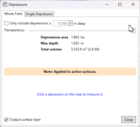
This tool displays all depressions in the visible surfaces. The overlay layer shows the depth of the depression with a white to blue scale, starting at white for zero depth, going to deep blue at maximum depth.

Tab: Whole Field

'☐ Only include depressions ≥ (X)m' allows you to filter out shallow depressions.
'Transparency' is a slider which adjusts how clearly the depressions will be displayed in the working area. With this, you can easily check the elevation surface underneath.
'☐ Output surface layer' controls whether the shown overlay layer will be retained when you click ‘Close’. If you are just checking their locations or volumes, you can untick it.

Statistics about the depressions found are displayed.

Tab: Single Depression

Clicking on a depression with this window open (from either tab) will switch to show this tab and show an outline on the map around the selected depression. This tab displays statistics about the selected depression: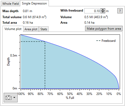

Left side:

'Max depth' This is the maximum depth of the selected depression.
'Total volume' This is the total volume of the selected depression, in your selected water and dirt volume units.
'Total area' This is the total area of the selected depression.

Right side:

'With freeboard' Freeboard is how far down the desired maximum water level is from the highest possible water level. For dams, this is usually chosen to reduce the risk of erosion leading to a breach or washout.
'Volume' This is the volume in the depression below the freeboard level. As freeboard increases, this will decrease.
'Area' This is the area of the depression at the chosen freeboard level. As freeboard increases, this will decrease.
'Make polygon from area' Click this to create a polygon from the outline on the map.

Further to the above statistics, detailed plots are available for more detailed analysis.

'Volume plot' The volume of the depression as a percentage of the total volume as it varies with depth is shown. The position of freeboard is indicated with a dashed line on the plot.
'Area plot' The area of the depression as a percentage of the total area as it varies with depth is shown. The position of freeboard is indicated with a dashed line on the plot.
'Stats' This sub-tab contains the information displayed in the volume and area plots. Click 'Copy Stats To Clipboard' copy it as text to the clipboard. The 'Separator' option allows changing the separator between values in the text. For copying to a spreadsheet, Tab is recommended.

The plots have a snapshot button in the lower left. Click it to see options to copy to clipboard or save to disk. You can also zoom in and on the plots using the mouse. Try scrolling on the main area or axes, dragging the mouse with different buttons held down, and remember that you can reset the view with double-middle-click.

Surface Derivatives

Show directional depressions

‘Show directional depression’ allows you to select a direction and display any depressions that would affect water flow in that specific direction that would otherwise not.

‘Direction (degrees)’ this setting will rotate the simulated water flow direction to help isolate depressions that would affect the water flow.
‘Plane strip width’ this tool performs its calculations in strips following the set direction, small strip sizes allow for a more detailed result but it takes longer to process.
The Compass is a visual method for controlling the direction that is used to calculate depressions.
‘Depressions deemed negative’ checking this option will tell the tool to display depressions as red on the surface.
‘Transparency’ controls how visible this information will be.
‘Output result layer’ will create an output layer upon closing the tool.
‘Apply’ this button must be pressed each time a change is made in order for it to be correctly displayed.

Surface Derivatives

Show watershed

‘Show watersheds’ identifies the areas of the surface that will flow together to the same exit point on a field. The working area will display the surface in a patchwork of colors, these indicate your watersheds and what will flow out where, the specific colors do not matter, they are only to help identify individual watersheds.

‘Elevation smoothing’ provides control to adjust the level of detail on the surface
‘Segmentation method’ will select a general water event to display watersheds. The options are:
- Hybrid - Immersion and Rainfall event happening simultaneously
- Immersion - submersion of the surface by water as it engulfs the area as in a flooding event
- Rainfall- a fall or shower of rain
‘Output watersheds layer’ will create a new design layer when the tool is closed.

Surface Derivatives

Show accumulated flow layer

The accumulated flow layer shows paths where the water is most likely to pass through. It is recommended that before using the ‘Show accumulated flow’ tool that the ‘Breach depressions’ tool is used for the most accurate water flow results.

‘Min. drainage area’ adjusts what the minimum drainage area needs to be before the paths will appear on the surface. The further to the left that the slider is the lower the amount of water that needs to pass through that area to appear on the field in the working area.
‘Transparency’ controls how the flow is displayed.
‘Output surface layer’ this will tell T3RRA Design Plus to create a design layer upon closing the tool.
‘Output flow paths’ which will create guidelines for the flow paths upon closing the tool.

Surface Derivatives

Show wetness index

‘Show Wetness index’ also referred to as the Hillslope Wetness Index. This tool creates a grayscale layer of the surface that uses high contrast to show the most affected areas. Darker areas on the field represent where the most water flow is, while lighter areas show where there is little water flow or where the water moves away from.

‘Elevation smoothing’ slider that averages out the information on the field reducing or increasing the number of peaks and valleys.
‘Transparency’ will change how visible the wetness index is.
‘Output result layer’ will create a design layer upon closing the tool.

Surface Derivatives

Show aspect

Showing aspect will change the surface to a gray-scale to highlight where the sun is hitting the surface. North facing areas will be lighter while south facing areas will be a darker gray.

‘Elevation smoothing’ slider that averages out the information on the field reducing or increasing the number of peaks and valleys.
‘Transparency’ controls how visible the layer is.
‘Output result layer’ will create an output layer upon closing the tool.

Surface Derivatives

Show slope

‘Show Slope’ shows the severity of the slopes in the field in a color grade. The color grade used is: Red shows low severity of slope and Dark Blue areas show a high severity of slope.

‘Elevation smoothing’ averages the information to grade how severe the slope is. The right end of the slider is the larger area averaged of the elevation points. The left side of the slider shifts the averaging to its smallest radius, resulting in slope severity to be more precise in which areas it reads.
‘Transparency’ which controls how visible the layer is.
‘Output result layer’ will create a new output surface upon closing the tool.

Surface Derivatives

Show directional slope

‘Show Directional slope’ allows you to visualize the severity of slopes going in a set direction. The severity of the slope is represented by color with Red showing a low severity of slope and dark Blue showing a high severity of the slope in that direction.

‘Direction (degrees)’, this setting allows you to set the directional slope you would like to see on the field. This is the manual direction setting which can be used if you know exactly which direction you wish to view.
‘Smooth elevation’ This slider manipulates the peaks and valleys in the present data by taking averages of the data around each point. The further to the right the slider is the more data is averaged resulting in fewer peaks and valleys present in the field.
The compass. The dark end of the compass needle represents the current directional heading you have set. To adjust the compass click and hold on the needle and rotate it to the direction you wish to display the slopes of.
‘Display back slopes as negative values’. This checkbox will display the slopes going in the opposite direction to the compass as a negative value, causing the field to appear vastly different.
‘Transparency’. This slider will change how visible the directional slope information is on the surface of the design.
‘Output result layer’ tells the system to create a surface layer when the pop-up window is closed.
‘Apply’. This button needs to be pressed each time you want to apply a new direction to the field.
‘Close’, this button will close the pop-up window and create a surface layer if the ‘Output result layer’ checkbox has been selected.

Surface Derivatives

Show landscape change

Landscape change is a large-scale smoothing operation for finding generalized high points.

‘Radius for gross landscape smooth operation’ this slider changes the radius for how far the system will look around each point to find the average height to be displayed.
‘Consider values higher than the average surface to be positive’ this option controls the color scheme of the display. If left unchecked, high points will be coloured red and low points will be dark blue and vice versa if the option is checked.
‘Perform exhaustive averaging (slow, but accurate)’ This slows down the averaging process but more closely analyses the information for more accurate adjustments.
‘Transparency’ controls how visible the changes of the tool are.
‘Output surface layer’ will create a surface layer upon closing the tool.

Boundaries Tools

Boundaries Tools Overview

When the Boundary tab is selected on the right hand side, the relevant tools will be accessed in two different areas. Firstly, on the menu bar (this changes depending on which layer type is selected) and is explained below in Boundary Design Tools and secondly, in the Layer menu on the selected tab and is explained in Boundaries Tools - Layer Menu.

Boundaries Design Tools

The Boundary tools available in T3RRA Design Plus create boundaries that are used to limit where field designs will affect. In order to apply any design to elevation data in T3RRA Design Plus they must first have a Boundary.

There are 5 Boundary tools available in T3RRA Design Plus, Point to Point Creation, Boundary Edit, Slice Boundaries, Multiple Cut lines and Open boundaries in Google Earth.

Boundaries Tools

Point to Point Creation

‘Point to Point Creation’ changes the mouse icon to a cross. While in this mode, clicking anywhere in the working area will add a point. These points anchor the line that appears on the screen with the last point and the first point connecting automatically to create a closed boundary line at all times. In order to complete and add the boundary to the layer selection, double click on the last desired point.

When creating boundaries, try to hug the surface fairly closely. Boundaries allocate memory for each pixel (blank ones too), so having extra space can slow down processing or cause out-of-memory errors.

Boundaries Tools

Boundary edit

‘Boundary Edit’ displays a series of nodes along existing boundary lines. By left-clicking and dragging these nodes, the boundary lines are able to be moved anywhere.

It is also possible to start editing a boundary by right-clicking on the map near it and choosing Edit nearest > Boundary.

To insert a new node in a boundary, hover over a line and left-click the blue node that appears. This inserts a new gray node to the boundary that can be further adjusted. Nodes can be removed by right-clicking on them.

Boundaries Tools

Slice Boundaries

‘Slice Boundaries’ is used to split pre-existing boundaries into smaller areas. Once this tool has been selected your mouse cursor will change to a pencil while it is in the working area. To add a line to a boundary click on the outside of the line to create a starting point, from this point wherever you move your mouse a red dotted line will be connected showing where the new boundary line will be created. Clicking on the working area again will place the new boundary line along the red dotted line that intersects with 2 other boundary lines.

Boundaries Tools

Multiple Cut lines

The ‘Multiple Cut Lines’ tool provides a way of creating equally spaced boundary lines across already existing boundaries.

When the tool is selected a pop-up window and a selection tool will appear in the working area.

In order to place the cut lines use the selection tool. The yellow square in the center of the selection tool controls the position of the lines, the yellow triangles on either side of the selection tool control the width of separation between the lines and the yellow circle controls the length of the selection tool as well as the rotation of the selection tool.

Boundaries Tools

Open Boundaries in Google Earth

‘Open Boundaries in Google Earth’ allows you to export your boundary lines to Google earth.

When the tool has been selected to export your boundary lines a pop-up window will appear. In this pop-up window the layer that is being exported can be named. Once the layer has been named press ‘OK’ and the layer will be exported to Google Earth.

Boundaries Tools

Boundaries Tools - Layer Menu

Open
Create
Edit
Create boundary from selected layer
Create region from selected layer - this will draw a region around the most outer points of the selected surface and will populate a new region in the Region tab
Merge selected - (ensuring you have 2 or more boundaries selected) this will create a combined boundary, removing the initial boundaries
Clean Selected
Copy selected - this will duplicate the selected boundary
Activate all - this will activate all the boundaries so they are visible on the Working Area. This is shown by the checkbox being selected.
Activate selected - this will activate the boundary which is selected (shown by the tile having a blue highlight around it) so it is now visible on the Working Area. This is shown by the checkbox being selected.
Deactivate all - this will deactivate all boundaries
Deactivate selected - this will deactivate the boundary which you currently have selected (shown by the tile having a blue highlight around it)
Delete selected - deletes the boundary that is selected (shown by the tile having a blue highlight around it)
Delete inactive - deletes all inactive surfaces (i.e. those without a tick in the checkbox)
Import >
- Import Shapefile
- Import KML
- Import Multiplane Boundary
- Import DXF points/linework
Export >
- Export selected to Shapefile
- Export selected to KML
- Export selected to Text Columns (CSV, TSV, etc)
View in Google Earth - this will open the selected surface in Google Earth
NOTE: You must have Google Earth Pro installed on your PC for this to work.

Regions Tools

Region Tools overview

When the Regions tab is selected on the right hand side, the relevant tools will be accessed in two different areas. Firstly, on the menu bar (this changes depending on which layer type is selected) and is explained below in Regions Design Tools and secondly, in the Layer menu on the selected tab and is explained in Regions Tools - Layer Menu

Regions Design Tools

Regions are a method of dividing a field or alike. Regions allow you to work with multiple fields separately in one project.

Regions Tools

Point to Point region creation

This tool lets you create custom regions. When using the creation tool, the cursor will change into a cross. Each left-click will add another corner to the closed region space. To finish adding points to the region, double-click where you would like the final point to be.

Regions Tools

Edit Region nodes and edges

This tool is used to make changes to an existing region. Start editing a region by right-clicking on the map near it and choosing Edit nearest > Region. Alternatively, select a region layer in the layers panel on the right then press the edit button. While editing, red dots are shown at each corner of the region. Each of the red dots can be dragged with the left mouse button to adjust the shape of the region.

To insert a new node, hover over a region line and click the blue dot that appears. The blue dot will turn red and become draggable. To remove a node, right-click it. To remove an edge from a region, right-click the edge.

Regions Tools

Split Region using Cut line

The ‘Cut line’ tool allows you to place a line to split a single region into two. This is useful when you wish to create different designs on different sections of the surface.

To use this tool ensure that you have an existing region selected in the layer selection.

To make a cut, left-click at one end of where you would like to cut and move the cursor to the other side. A red dotted line will appear along where the line will be cut. Make sure that this line intersects with at least two other lines of the existing region. When you are sure about the placement of the line left-click on the ending point to cut the region. Right-click to cancel the region cut.

Regions Tools

Region Multi-Slicer

The region multi slicer makes it easy to slice a region into many smaller ones. All cuts made with this tool will follow the same direction and will be parallel to each other.

To use this tool, make sure that you have a region layer selected.

When the tool is selected, it will automatically generate a set of lines. The yellow anchor points can be used to edit the size and positioning of the slices.

‘Strip width’. This value controls how far apart each line is. This option allows for precise control over the width.
‘Strip count’. This value controls the number of lines that will be used to cut the field.
‘Segment length’. This option controls the length of the lines used to cut the region. Adjusting the value here has the same effect as moving the yellow circle anchor.
‘Total width’ and ‘Total length’ are not adjustable options − they are for display only, and are calculated from ‘Strip width’ and ‘Segment length’.
‘Bearing’. This option is a more precise method of adjusting the heading of the lines. The ‘East/West’ and ‘North/South’ buttons set the heading to follow directly along those directions.

Once all changes have been made, press the ‘Apply’ button to make the cuts on the selected regions, or the ‘Cancel’ button to back out of this tool.

Regions Tools

Regions Tools - Layer Menu

Open
Create >
- Create from saved surface
- Create from selected surface
- Create from saved boundary
- Create from selected boun
Edit
Create boundary from selected layer
Create region from selected layer - this will draw a region around the most outer points of the selected surface and will populate a new region in the Region tab
Merge selected - (ensuring you have 2 or more boundaries selected) this will create a combined boundary, removing the initial boundaries
Clean Selected - See below
Copy selected - this will duplicate the selected boundary
Activate all - this will activate all the boundaries so they are visible on the Working Area. This is shown by the checkbox being selected.
Activate selected - this will activate the boundary which is selected (shown by the tile having a blue highlight around it) so it is now visible on the Working Area. This is shown by the checkbox being selected.
Deactivate all - this will deactivate all boundaries
Deactivate selected - this will deactivate the boundary which you currently have selected (shown by the tile having a blue highlight around it)
Delete selected - deletes the boundary that is selected (shown by the tile having a blue highlight around it)
Delete inactive - deletes all inactive surfaces (i.e. those without a tick in the checkbox)
Import >
- Import Shapefile
- Import KML
- Import Multiplane Boundary
- Import DXF points/linework
Export >
- Export selected to Shapefile
- Export selected to KML
- Export selected to Text Columns (CSV, TSV, etc)
View in Google Earth - this will open the selected surface in Google Earth
NOTE: You must have Google Earth Pro installed on your PC for this to work.

Clean Selected explained

Clean selected attempts to simplify and clean the regions by combining points that are very close together (<1mm). It also occurs when dragging nodes and splitting.

In general splitting and editing regions will attempt to reduce the number of points in the region by detecting points that end up close to each other. This can be really helpful when creating internal voids in a region. To do so, add 3 points on the edge of a region, then drag the middle one to where you want your void. Add points near the middle point to go around the void. Then drag the last point you add right on top of the 'middle' point (you may need to zoom in to get it close enough). When you are prompted to simplify/combine, choose Yes. Combine the two points at the edge in the same way. Now you have an internal void.

Guides Tools

Guides Tools - Overview

The ‘Guides’ layers allow extra information to be displayed on the field in the working area. This information can include elevation grids, flow directions, and contour lines.

There are many tools available in the guides toolbar to help manage and quantify the elevations on the field.

Guides can also be exported in control files for use in T3RRA in cab software (e.g. T3RRA Cutta) by dragging them into the export window. See more in Exporting a T3RRA Cutta (*.tci) Control File.

Guides Tools

Edit Guide

The ‘Edit guide’ tool allows you to make changes to the selected guide. To edit a guide, right-click near it on the map and select Edit nearest > Guide, or select it in the layers panel on the right and press the ‘Edit Guide’ button. While editing, the guide’s window will open.

Guides Tools

Point Label

This tool lets you place labels on a field as reference points, or simply to remind you of points you may need to watch out for or pay closer attention to. Selecting the tool will change the mouse cursor to a cross. Clicking in the working area with the cross will create a point and open a pop-up window, allowing you to edit its properties:

‘Label’ The text in this box will be displayed on the map. The size of the text can be altered by using the ‘Text size’ option on its right.
‘Symbol’ allows you to change the symbol or shape that is used for the point.
‘Symbol size’ allows you to make the symbol larger or smaller.
‘Color’ allows you to change the color of the label marker that is placed on the field in the working area.
‘Use this label as sub-region title’ affects the printed output. When selected, will use the label as the title for the region part it is in. It is only applicable when region-parts are set to output when printing.
Easting and Northing show the coordinates of where the point label has been placed. It can be changed using the yellow point on the marker or by inputting new values here.
‘Value’ option displays the elevation or height of the label and can be changed by entering a new value here. If you enter a custom value, ensure you lock it with the neighboring option.
‘Lock value’ locks the value that has been set in the ‘value’ field so that it will not update to the currently active surface. Unlocking a point label is a way to get a surface elevation of cut/fill value at a specific point.
Clicking on the ‘Copy to clipboard’ button will copy the name of the label and its coordinates so they can be used elsewhere.

When creating a label, if you have a label layer selected on the right, it will be added to that layer (otherwise it will create a new layer for it).

Guides Tools

Line Label guide

The ‘Line Label guide’ tool allows you to select two points anywhere on the field and display the distance between them with a label attached. When the tool has been selected the cursor will change into a cross.

‘Label’ This is the title of the line that has just been created. The label’s text size can be changed using the ‘Text size’ option to its right. This text size option will only affect the title on the guide, it will not increase the size of the text in the measurement.
‘Line style’. The left drop down menu allows you to change the color of the line, the right drop down menu allows you to select the thickness of the line.
‘Arrow at start’ and ‘Arrow at end’ allow you to add arrows to the start and end of the line.
‘Show distance’ adds a secondary, thinner, line below the original line that displays the distance covered by the line. This option is turned on by default.

Guides Tools

Circle guide

The ‘Circle guide’ tool will display the radius and total area covered by the set circle. To use the tool, left click where you want the center of the circle to be and drag the mouse until the circle is at the desired size.

The option on the left in the window allows you to select the color of the circle. The option on the right allows you to select the thickness of the line.

At the center point of the circle, the total surface area of the circle is displayed. Starting from the same central point, a radius line will be placed showing the distance of the center to the edge of the circle.

Guides Tools

Strip/Corridor guide

The ‘Strip/Corridor guide’ tool creates 2 parallel lines. When selecting this tool, click on the field where you would like the center point of 1 line to be, then drag away from this point to create a set of parallel lines.

‘Width’ displays the current width set between the lines. The distance between the lines can be adjusted by typing a new value here or by moving the yellow triangle on the surface.
‘Length’. Changing the length value adjusts the size of both lines. The length may also be adjusted by dragging the yellow circle point that is at the end of one of the lines.
‘Line style’. The left menu allows you to select the color of the lines, while the right menu lets you select line thickness.
‘Arrow at start’ and ‘Arrow at end’. Selecting either of these checkboxes will create arrows at their respective location on the lines.

Guides Tools

Polyline measurement

The ‘Polyline measurement’ tool is used to create a guide line with multiple segments. The length of individual segments and the angles between them may also be displayed. When the tool has been selected, the cursor will change into a cross. Left clicking anywhere in the working area will place the first point, and clicking again will place segments. To finish adding segments, double click on the final point. Double clicking will open a window where settings for the polyline can be changed. The points of the polyline can be adjusted by dragging the yellow squares.

‘Line style’. The left drop down menu lets you set the line color, while the right drop down menu lets you set line thickness.
‘Smooth’ will take the points that are available and adjust them to a more direct path with fewer corners. When the slider is all the way to the right, the points of the measurement guide will be lined up in a straight line.
‘Simplify’ will remove points along the polyline while attempting to follow the original path as closely as possible. This is most visible when the slider is used on polylines that make small direction adjustments.
‘Use real unit width’ when selected will disable the right drop down menu of ‘Line style’ and set the width to the value on the right of the checkbox. When using this option, the line thickness is no longer linked to pixels and will increase in size as the zoom level increases.
‘Show distances’ will display the length of each segment of the polyline.
‘Show angles’ will display the inside angles of each joint between segments.
‘Show slopes’ will display the overall grade of each segment as a percentage.

Guides Tools

Polygon measurement

The ‘Polygon measurement’ tool measures the length of the sides as well as total space covered inside a chosen shape. When selecting the tool, the cursor will change into a cross. Clicking on the working area will place a point − continue clicking where you would like points to be placed, and double click on the final point to finish placement. The yellow squares can then be dragged around to adjust the shape.

‘Line style’. The left drop down menu lets you select the color of the guidelines. The right drop down menu allows you to change the thickness of the guidelines.
‘Fill style’. The left drop down menu allows you to set the color of the shape’s fill. The right drop down menu provides 3 options as to how the closed shape will be filled: a solid color, a hatched pattern, or a dotted pattern.
‘Show distances’. Sets whether the distance of each segment is displayed. There are two options to the right to control where they are displayed.
‘Show angles’ will toggle on and off the display of angles between each segment of the polygon guide.
‘Show area’. This option toggles on and off the value shown at the center of the polygon.
‘Text size’ controls the text size of the total area covered − it does not affect the text size of the distances and angles.

Guides Tools

AB lines

The ‘AB lines’ tool creates a pattern of guides along the working area. When using the tool, the cursor will change into a cross. Click on two points in the working area to create an AB line.

‘Heading’. The value in the heading setting controls the direction of the guidelines. The value displayed is the heading in degrees of Point B from Point A.
‘Swath width’ controls how far apart the lines are. The two dotted lines (on either side of the central line) show the reach of the implement (its swath width) as it travels down the first/central AB line. Thes can be used to position the first line relative to a boundary, or other feature.
‘Swath distance format’. This setting changes how the line labels are displayed.
- ‘Distance’- will label each line as how many meters it is from the center line.
- ‘+/-’ - will label each line as a number and whether it is positive or negative.
- ‘L/R’ - will label each line a number and either L or R depending on which side of the center line it is.
- ‘None’ will remove all labels from the AB lines.
‘Line style’. The left drop down menu will let you set the color of the guidelines, while the right drop down menu will let you set the thickness of the guidelines.

Guides Tools

Elevations Guide

The ‘Elevations guide’ imposes a grid design on a field in the working area and displays the elevation of points at each junction on the grid. When using this tool the cursor will become a crossClicking on the working area in the desired center point will create a grid. The grid size and position can be manipulated by using the yellow anchors.

‘Grid cell size’. This option controls the size of the grid. Setting the size to 100m will result in each junction being 100 meters away from its neighbors.
‘Alignment angle’ is a method of rotating the grid.
‘Text size’. This option is a drop down menu that allows you to change the text size of the values on the grid.
‘Decimal places’. Sets how many decimal places will be visible on the grid values.
‘Show elevation’, ‘Show offsets from mean elevation’, and ‘Show offsets from center elevation’. These options will adjust what data is present on the grid.
‘Use topmost layer’, ‘Use selected layer(s)’, and ‘Use all surface layers’ control which surface layer is used to calculate the elevation points on the grid.
‘Display units’. By selecting this checkbox, the measurement units (meters, feet) will be shown on each value on the grid.
‘Auto-update surface changes’. By selecting this checkbox the grid will automatically update the displayed values when surface layers are changed.
The grid is able to be exported into a CSV format by pressing the ‘Export to CSV’ button in the bottom right of the pop-up window.

Guides Tools

Flow direction guide

The ‘Flow direction’ guides creates a grid on the field with arrows at each junction that point in the direction that water is expected to flow. When the tool is selected the cursor will change into a cross, and left-clicking in the working area will create a grid centered where you clicked.

‘Grid cell size’. Adjusting this value will make the individual squares of the grid larger or smaller.
‘Grid alignment angle’. This option allows you to change the direction of the grid.The direction is set as the position of the yellow circle in relation to the yellow square.
‘Slope calculation area’. The further to the right that the slider is, the larger the area that T3RRA Design Plus takes as a sample to find the water flow direction.
‘Line style’. The left drop down allows you to change the color of the arrows on the field. The drop down menu on the right allows you to adjust the thickness of the arrows.
‘Auto-update with surface changes’. When this option is selected, the grid will automatically update when the surface layer changes.

Guides Tools

Contour lines

The ‘Contour lines’ tool allows for the automatic creation of contour lines on the selected field. When the tool is selected, the cursor will change into a cross. Left-clicking on the desired field will generate contour lines and open a pop-up window that allows you to make changes to the contour lines.

‘Reference elevation’ allows you to change the starting elevation that contours fan out from.
‘Vertical interval’ is used to change the elevation change between contour lines.
‘Smooth contours’. This slider will smooth out sharp turns in the lines. The further to the right the slider is, the more smoothed the contour lines will be.
‘Simplify contours’. This slider adjusts how complex the lines are. The further to the right the slider is, the straighter the lines will become.
‘Show labels’. On the left is a set of 3 choices: ‘contour altitudes’, ‘line numbers’, and ‘no labels’. These options control the display of information on each contour line. ‘Contour altitudes’ will display the elevation of each contour line. The second choice, ‘line numbers’, will display the number of each line, starting from the reference line. The final choice is ‘no labels’, this choice will leave the lines unlabeled.
‘Min. contour size’ is the minimum length of contour lines placed on the field.
The ‘Contour line size’ options are a set of drop down menus. The left menu lets you select the color of the contour line, and the right menu lets you choose line thickness.
‘Label size’ will adjust the size of text along the contour lines.

Guides Tools

Slope Indicator

The ‘Slope Indicator’ tool is used to measure the slope of a particular area. When the tool is selected the cursor will change into a cross. Once a point has been selected, slope indicators will appear on the field and a pop-up window will be opened. The slope indicators can be manipulated on the field by using the yellow anchor points.

‘Base point latitude’ and ‘Longitude’. These options control the position of the indicator on the field. They can be manually changed by typing new values in the boxes. These changes take immediate effect.
‘Main angle’ This option controls the direction of the main direction line. The line changes size proportionally to the slope of the area. Until the settings have been finalized, the direction of the main line can be modified with the yellow circle anchor.
‘Area size’. This option controls the sample area of the slope indicator. The elevations within the sample area are read to determine the displayed slope. Increasing the value displayed in the box reads more elevations and provides a more averaged slope measurement. Decreasing the area size gives a more specific and local slope measurement.
‘Side angle’ and ‘Max. slope angle’ cannot be changed directly - they display the secondary heading and the heading of the maximum slope at the selected location.
‘Reference line length’ allows you to change the maximum length of the slope indicators.
‘Lock reference line length’. When selected, this locks the reference line to its current length while dragging the yellow circle.
‘Show line lengths proportional to line slopes’. When selected, the lines will adjust in length to match the slope of the selected area. They will not exceed the reference line length.
‘Hide primary and secondary direction lines when not editing’, selecting this option will hide the main direction line and the secondary direction line once all settings have been finalized and the window has been closed.
‘Main/side line style’ the left drop down menu lets you select the color of the two slope lines at 90° to each other. The right drop down menu lets you select their thickness.
‘Max. slope line style’ the left drop down menu allows you to change the color of the maximum slope line. The right drop down menu allows you to change the thickness of the slope line.
‘Separate indicator from reference point’. This option allows you to move the indicator to another location while still using the same reference point. Once settings have been finalized the reference point and area will be invisible.
‘Use this slope for print output’. This option selects this slope for printing output.
‘Auto-update with the surface changes’. This check box will cause the slope indicator to adjust the displayed values depending on the top most layer in the surface selection.

Guides Tools

Create flow paths

The ‘Create flow paths’ tool is used to create a display of the likely water paths present in a field. When the tool is selected, the cursor will change into a cross. Left click on a field to display the flow paths. Once a field has been selected, it will be populated with flow lines and a pop-up window will be opened.

‘Elevation smoothing’. This option is a slider that controls the smoothing of the elevation before creating the flow lines. The further to the right that the slider is, the more imperfections are taken out of the flow paths, creating straighter paths.
‘Seed points grid size’ controls the size of the grid that is used to take samples for flow paths. Setting a higher value here makes a larger grid and hence takes fewer samples.
‘Flow path style’ is a set of 2 drop down menus. The left drop down menu sets the color of the flow paths, by default this is set to black. The right drop down menu sets the thickness of the flow paths, by default this is set to the thinnest option.

In order for any changes made in the window to be reflected in the field you need to press the ‘Apply’ button at the bottom of the window. Once all desired changes have been made press the ‘Close’ button on the window to save all changes.